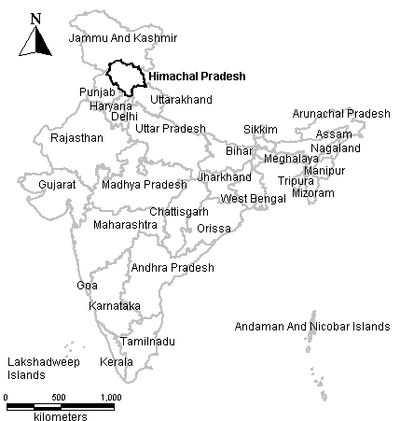
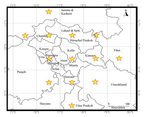
Abstract

Estimation of solar energy reaching the earth’s surface is essential for solar potential assessment, design of solar energy based applications, meteorology, climatology, oceanography, agriculture, forestry and for many other domains. Global insolation measured using data obtained from satellites provides higher spatial and temporal coverage of regions compared to ground based data from radiation stations or models based on other meteorological parameters.  Solar potential of the Indian hill state of Himachal Pradesh has been assessed using NASA’s Surface Meteorology and Solar Energy (SSE) data over 1°x1° global grid for 22 years. Monthly global insolation contour maps have been computed through interpolations and Geographical Information System (GIS). The results have been validated with ground data (Root Mean Square Error of 4.88%). Influences of seasons, meteorological parameters and topography on global insolation have also been analysed. It is observed that, during the period of March to October, the state receives global insolation above 4 kWh/m²/day throughout its eclectic topography with a peak of ~6.84 kWh/m²/day seen in the months of May and June encouraging viable solar devices. However high altitude regions such as of Kullu, Kinnaur and Lahul Spiti, have lesser global insolation below 4 kWh/m²/day with a minimum of 2.57 kWh/m²/day during winter months of November - February. Compared to this, low and medium altitude regions receive an average global insolation of  ~ 4.5 kWh/m²/day during November - February and lesser than high altitude regions during December and January.
Keywords: Solar potential assessment, Himachal Pradesh, India, Global insolation, Spatial data, Geographic Information System (GIS), Geoinformatics, Renewable Energy

Introduction

Energy plays a pivotal role in the development of a region. However, energy shortages in recent times, the imminent energy crisis and threat of climate change have focused the attention for a viable sustainable alternative through renewable sources of energy. Sun is the vital source of energy manifested in different forms in the solar system. Solar energy intercepted by the earth at the rate of 1.7 X 1014 kW is many times greater than its present rate of overall energy consumption. Approximately 99% of the solar energy is contained in the wavelength band of 0.15 - 4.0 µm consisting of the ultraviolet, visible and near infrared regions of the solar spectrum. The geometry of the earth-sun movements causes large spatial, diurnal and seasonal variations in the amount of solar radiation received on earth. The 23.5° tilt of the earth’s rotational axis with respect to the plane of orbital revolution causes larger annual variations near the poles and smaller variations near the equator [1]. Due to the variations in the sun-earth distance, intercepted solar radiation fluctuates by ±3.3 % around its mean value. The variations due to sunspots, prominences and solar flares, can be neglected as they constitute small fraction compared to the total energy emitted by the sun. The average solar radiation falling on the earth’s atmosphere called the solar constant is estimated to be 1.36 kW/m2. The presence of clouds, suspended dust, gas molecules and aerosols in the atmosphere, through absorption and scattering, attenuates the incident solar energy radiation (also called insolation). A fraction of 0.3 of the total incident solar energy called the albedo of the earth-atmosphere system is reflected back to the space [2]. The remaining fraction of solar energy in the form of direct and diffuse insolation which comprises the global insolation is utilized in many processes like heating and illuminating the earth, photosynthesis, growth of vegetation, evapotranspiration, snow ablation as well as solar energy based applications. Solar radiation data is essential for solar energy potential assessment for designing solar energy based applications, meteorology, climatology, oceanography, agriculture, forestry and many other domains. Solar energy applications like photovoltaic based off-grid and utility grid power generation, solar water heaters, thermal concentrators, solar cookers, desalination plants, passive building heating etc. demand reliable information on surface global insolation measurements at different regions of interest. This could be estimated from insolation data procured from on-ground pyranometric networks, models based on meteorological parameters or those based on satellite data.

Solar potential assessment

Insolation data from pyranometric networks: Conventionally, solar potential of a region has been assessed using the insolation data obtained from ground based radiation stations. There are more than 500 radiation stations in 56 countries which provide global, diffuse and direct insolation data on hourly, daily or monthly basis to the World Meteorological Organisation apart from other archived data from radiation stations around the world [3]. An efficient and reliable pyranometric network, incurs heavy investment in terms of capital, maintenance and manpower. Developing countries like India with a vast land area of 3287263 km2, find it hard to have a sufficient spatial coverage for insolation measurements. The Indian radiation network under the Indian Meteorological Department (IMD) has merely 43 radiation stations spread across the country. Data from ground based solar radiation monitoring stations are liable to errors due to calibration drift, manual data collection, soiling of sensors and non-standardization of measuring instruments [4]. The World Climate Research Program in 1989 had estimated an end to end uncertainty of 6% -12% in measurements from common solar radiation stations [5]. Most of the data available from radiation stations are at non- uniform and interrupted periods as shown by Alberto Ortega et al [6]for Chile which was reported to be 3 months to 21 years. In the case of India, its radiation network expanded from 4 stations in 1957 to 43 as of today, measuring one or more parameters like Global, Direct or Diffuse radiation at different locations.  These datasets provide temporal information (in minutes) which are essentially important for solar energy applications and design [7]. Annual insolation varies with change in angle of incidence of the solar radiation. It is reported that a minimum of 7-10 years of solar radiation data is required to get a long term mean within 5 % [8].

Insolation data from meteorological parameters: Insufficient insolation data consequent to sparse radiation networks, lead to different parametric (Iqbal and ASHRAE Model) and decomposition models (Angstrom, Hay, Liu and Jordan, Orgill and Hollands Model). These models employ theoretical or empirical methods for interpolation or extrapolation of measured meteorological values to derive insolation data [1].These models use parameters like sunshine duration [9, 10], temperature [11], rainfall [12], cloud cover [13], extraterrestrial radiation [14], etc.  for estimating solar radiation over a given location. Artificial Neural Networks (ANN) have also been utilized for deriving insolation data based on climatological and geographical parameters [15]. These methods show low Root Mean Square Errors (RMSE) of 5% on validation with in-situ measurements and still are inadequate for large spatial and temporal scale studies.

Insolation data from satellites: Remote sensing data from polar satellites at ~850 km with higher spatial resolution and geostationary satellites at ~36000 km with higher temporal resolution are being utilized for different studies[16]. The LANDSAT – MSS/TM, SPOT – VHR, NIMBUS – CZCS, NOAA – AVHRR, INSAT- VISSR, GOES –VISSR instruments [17] provide information for estimation of insolation based on different subjective, empirical and theoretical methods.

Subjective methods involve subjective interpretation of cloud cover from the satellite images and its statistical relationship with atmospheric transmittance. Empirical methods depend on functional relations based on satellite derived data and available solar radiation data which are customized for any place and time. Empirical methods are classified into two models: statistical and physical. Statistical models use independent variables including brightness levels, solar zenith angle, precipitable water and cloud amount inferred from satellite data on the basis of their ability to explain the variability in solar radiation. They depend on ground networks for parameterization and do not require satellite sensor calibration. Physical models are originated from the radiation balance of the earth atmospheric system. They deduce surface insolation by physical simulation of radiation transfer through the atmosphere and are independent of the ground data while demanding sensor calibration. Another method which simulates radiant energy exchanges taking place within the earth atmospheric system, hypothetically not demanding empirical calibration of model parameters is called theoretical method. The broadband and spectral models are attached to this method [18].

The solar potential of Kampuchea was estimated based on a statistical model [19] with the visible and infrared images obtained from Japanese Stationary Meteorological Satellite GMS-3 along with ground based regression parameters and concluded that seasonal average of daily insolation depended more on the topography of the region than on seasonal variations. The Root Mean Square Error (RMSE) of the monthly average insolation were shown to vary from 5.7% to 11.6% as the cloudiness of the region increased. The solar potential of Pakistan was estimated by employing a physical model [17] based on the images collected from the Geostationary Operational Environmental Satellite (GOES) INSAT which scanned the region four times per day. The results indicate that the desert and plateau regions received favourable global insolation while the monsoon had its influence on reduced insolation in the eastern and southeastern Pakistan, for the months of August, October and May.  

Daily global insolation in Brazil was assessed for cloudy, partially cloudy and clear sky conditions based on a statistical model on images from GOES- VISSR instrument and verified it to obtain standard errors of 27%, 15% and 11% respectively [20].  Attempt was made to obtain a reliable solar map for Chile [6] based on a physical model applied to the GOES-8 and GOES-12 images validated with the ground data. They reported regional and temporal variations in global insolation due to the diverse topography and climate of Chile. Stretched Visible Infrared Spin Scan Radiometer (S-VISSR) images of Geostationary Meteorological Satellite (GMS) of 15 minute interval high spatial resolution (0.01⁰X0.01⁰) for a period of 3 months in 1996 [21] were analysed to develop a bispectral threshold technique with respect to earth-atmosphere albedo and infrared temperature and performed a parameter tuning of the model at 67 weather stations. It was shown that more the number of higher resolution images used, lower is the Root Mean Square Error (RMSE) of hourly insolation compared to ground data and was more evident for regions with rapid variations in insolation due to topography. The RMSE was calculated to be 25 % for daily and 12% for hourly insolation data obtained. Similar endeavor generated hourly and monthly basis global as well as direct insolation maps using SOLARMET physical model applied over 7 years high resolution Meteosat satellite images [22]. They also employed a smoothing procedure over each 3X3 km pixels so as to obtain regular insolation contour lines over the maps produced. It was found that the modeled insolation data showed a yearly average relative difference of 7.6% when compared to the data from 51 ground stations. A physical model based on visible range satellite images considering the climatological aspects of hourly global insolation useful for designing solar energy systems was designed [23]. The importance of aerosols in solar radiation depletion has been studied and a method to address it in the model is discussed. The model is specifically applicable for tropical regions like South East Asia and Thailand is taken as the study area. In the study, 8 years 3X3 km resolution GMS 5 visible images are used to obtain monthly average hourly insolation datasets with RMSE ~10% when validated with 25 pyranometric stations. Evaluation of the direct beam insolation in Abudhabi for a year is about 400W/m² based on the monitored ground data [24]. This data was validated with the 22 year average data from NASA’s Surface Meteorology and Solar Energy (SSE) datasets, which proved that the region was a high potential area for solar energy based applications. Satellite-data based models do not show much difference in performance as the primary source of ambiguity for all these models is the influence of cloud pattern. It has been proved that interpolations and extrapolations of available ground data for predicting solar radiation over distances beyond 34 km show higher RMSE compared to satellite-data based measurements [25]. RMSE for different models have been found to be within 20% for daily values and 10% for hourly values [26]. Today satellite data for about 20 years are available, which reduces the possibility of error due to annual variations in insolation. Nevertheless, ground data is indispensable at this juncture for validation and model improvement of satellite based data.

Objective

The prime objective of this study is to assess the solar energy potential of the Indian federal state of Himachal Pradesh using higher spatial and temporal scale satellite derived monthly average global insolation datasets.

Study area

Geography and climate
Himachal Pradesh (Figure 1) is located between 30.38° to 33.21° North latitudes and 75.77° to 79.07° East longitudes, in the western Himalayas, covering a geographical area of 55673 km2. The State is divided into 12 districts surrounded by Jammu and Kashmir in the North, Tibet in the Northeast, Uttarakhand in East/Southeast, Haryana in South and Punjab in Southwest/West, with an abundance of snow fed perennial rivers and rivulets. Out of the total area, 37,033 km2 is managed by the forest department and 16,376 km2 is under permanent snow cover [27].

Figure 1: Study area - Himachal Pradesh, India

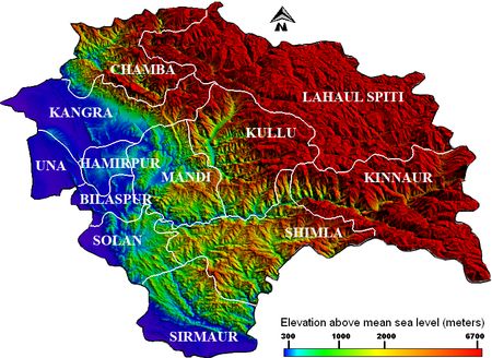
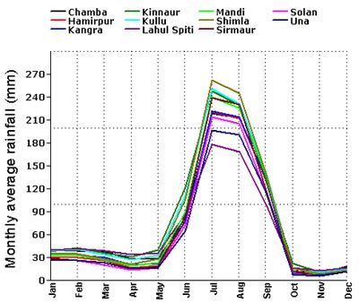
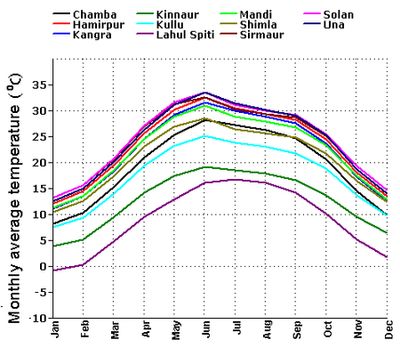
The agro-climatic zones of Himachal Pradesh are divided based on its elevation above mean sea level. Parts of Una, Bilaspur, Hamirpur, Kangra, Solan and Sirmaur districts in the Western and Southern regions lie below 1000m with a tropical climate and respective vegetation. Some portions of Solan, Sirmaur, Mandi, Chamba and Shimla districts at altitude between 1000-3500 m have climate conditions varying from sub-tropical to wet- temperate with elevation. Lahaul Spiti, Kullu and Kinnaur districts ranging between 3500-6700 m are part of the dry temperate, sub-alpine and alpine zones with very sparse rainfall of less than 80cm annually. The Digital Elevation Model (DEM) of the state provides a clearer understanding of its topography (Figure 2).

Figure 2:  Digital Elevation Model of Himachal Pradesh

The spatial and monthly variations of average rainfall (Figure 3) and temperature (Figure 4) over Himachal Pradesh have been observed from a 100 years meteorological dataset. The monthly average temperature decreases with altitude and shows a regional difference of approximately 15° C from higher elevations (above 3500 m) to lower (below 1000 m). Winter season commences in the month of October, reaches its peak in January and continues till February. The months of March, April, May and June are comparatively warmer. Figure 3 clearly shows the onset of Southwest monsoon in June with average rainfall uniformly reaching higher values in all the regions. The highest annual average rainfall is recorded in the district of Kinnaur and the least in Una. The rainfall slows down towards the end of September marking the end of the southwest monsoon season.

Figure 3:  Monthly average rainfall variation in Himachal Pradesh

Figure 4: Monthly average temperature variation in Himachal Pradesh

Availability of ground radiation data

Himachal Pradesh has an IMD’s ordinary radiation station which is situated in Manali at 32.27° North latitude and 77.17° East longitude measuring gobal insolation. The data from the station do not suffice for a higher temporal and spatial scale study of solar energy availability throughout the state. Hence 22 year average satellite data with 1° X 1° resolution have been used apart from validating with ground based estimations. 

Data and methodology

Data source
Surface Meteorology and Solar Energy (SSE) datasets provided by the National Aeronautics and Space Administration (NASA) Langley Research Center give solar radiation and meteorological data collected by a variety of earth-observing satellites from different countries. These datasets are global and contiguous in time and are accessible (http://gewex-srb.larc.nasa.gov) in user friendly formats. The solar radiation parameters were validated with the Baseline Surface Radiation Network (BSRN) while the meteorological parameters were validated with the National Climate Data Center (NCDC). SSE data was validated with BSRN data (RMSE 10.28% for global horizontal insolation). SSE Release 6.0 datasets of 2008 were used for this work. The data is of spatial resolution of 1°x1° on a global grid and temporal coverage of solar radiation parameters for 22 years from July 1st, 1983 to June 30th, 2005 [5].

Model
The SSE datasets are derived from a physical model based on the radiative transfer theory employing a modeled atmosphere along with parameterization of its absorption and scattering properties. Primary inputs to the model include visible and infrared radiation, inferred cloud and surface properties, temperature, precipitable water, column ozone amounts and atmospheric state variables such as temperature and pressure [28]. The parameters have been measured using instruments like CERES (Clouds and the Earth’s Radiant Energy System), MODIS (Moderate-resolution Imaging Spectro Radiometer), TOMS (Total Ozone Mapping Spectrometer) etc mounted on GMS, NIMBUS, METEOR, GOES, METEOSAT, NOAA and many other satellites. Insolation at a given location on the earth’s surface is inferred based on the shortwave (0.2 to 4um) and longwave (4 to 100um) solar radiation reflected to the satellite sensors from the Top of Atmosphere (TOA). A calculative TOA solar radiation is iteratively compared to the values measured by the satellite sensors. Iterations are carried on parameters like aerosol distribution until the error is within a marginal value. Global insolation on the surface for each such iteration is also computed. This forms the dataset for global insolation incident on a horizontal surface for given durations [5].

Shortwave and longwave solar radiation datasets were derived (discussed in the next section) based on primary algorithms by Pinker and Lazlo (1992) and Fu et al (1997) respectively. The quality check algorithms called the Langley Parameterized Shortwave Algorithm (LPSA) and Downward Longwave Algorithm by Gupta et al (2001 and 1992 respectively) validates the primary algorithms [29]. All the released datasets in SSE have undergone validation based on these four algorithms. Here we have discussed the quality check algorithms which forms the foundation for shortwave and longwave datasets.

Shortwave algorithm: The LPSA by Gupta et al [30]gives the downward shortwave flux as

F_SD =F_TOAT_AT_C                                                                                                       …….. (1)

where FTOAis the corresponding shortwave insolation at the TOA, T_A is the transmittance of the clear atmosphere,  and T_c is the transmittance of clouds in which all parameters are computed on a daily average basis.

Insolation at TOA is given by,

F_TOA= S(d_m/d )² cosZ                                                                                   ......... (2)

where Sis the solar constant, dis the instantaneous Sun-Earth distance, d_m is the mean Sun-Earth distance and Z is the solar zenith angle.

Clear-sky transmittance is given by,

T_A = (1+B)e ^-τz                                                                                                          ……..(3)

where the term B accounts for the reflected solar radiation from the surface that is backscattered by the atmosphere (calculated with surface albedo as a parameter) and τz accounts for all absorption and scattering properties of gases and aerosols in the clear sky.

Cloud transmittance Tc is given by, 

Tc= 0.05 + 0.95 (R_ave – R_meas)/(R_ave – R_clr)                                                                        …….(4)

where R_ave, R_clr and Rmeas represent daily average values of overcast, clear and measured reflectance respectively, corresponding to an overhead sun. Even for the thickest clouds Tc is not reduced to zero.

Longwave algorithm:  Based on the quality check algorithm by Gupta et al [31]the surface downward long wave flux is given by

F_LD = C₁ + C₂A_c                                                                                             ……….(5)

where C₁ is the clear sky flux, C₂ is the cloudy sky flux (also called cloud forcing factor) and Ac is the fractional cloud cover. C₁ and C₂ are parameterized based on radiative transfer calculations on a range of meteorological inputs. While C₁ is calculated over total precipitable water and effective emitting temperature of the atmosphere, C₂ is a function of total water vapour content and temperature at the cloud base for the layer considered.

Data Procurement
The global insolation data for horizontal surfaces are available as daily, monthly and annual averages obtained from daily 3 hourly datasets for UTC (Coordinated Universal Time) 0, 3, 6, 9, 12, 15, 18, 21 hrs on any 1° X 1° global grid from the SSE web portal. Within a 1° X 1° grid, any points which do not lie on its Northern or Eastern boundaries share a common insolation value corresponding to the midpoint of the grid. The study area of Himachal Pradesh lies between 30.38° to 33.21° North latitudes and 75.77° to 79.07° East longitudes. Out of 13 optimal grids (regions) from 29.5° to 33.5° North latitudes and 75.5° to 79.5° East longitudes (Table 1) , 10 grids provide a complete coverage of the land area of the state while the other 3 are used to support an optimal interpolation through Geographic Information System (GIS). Out of the 13 selected grids, 6 grids cover Chamba, Lahaul-Spiti, Krishnaganj/Kinnaur, Hamirpur, Kullu and Sirmaur districts of Himachal Pradesh, 5 grids cover the districts of Kargil, Kathua (Jammu & Kashmir), Fatehgarh Sahib (Punjab), Muzaffarnagar (Uttarpradesh), Tehri Garhwal (Uttarakand) and 2 grids cover the Tibetan region (Figure 5).

Figure 5: Selected regions (star marked) for obtaining monthly average insolation maps in GIS

Results and discussion

The average global insolation datasets of 22 years (Table 1) were analysed spatially using GIS to understand monthly global insolation variations. Season wise analysis show that Himachal Pradesh receives an average insolation of  5.99 kWh/m²/day in the warm summer months of March, April and May; 5.89 kWh/m²/day in the wet monsoon months of June, July, August and September; 3.94 kWh/m²/day in the colder winter months of end October, November, December, January and February. It is observed that the period from March to October which covers the summer and monsoon seasons, over the entire physiographic zones of Himachal Pradesh receives insolation above 4 kWh/m²/day. This indicates favourable solar potential for commercial as well as domestic energy applications. The insolation throughout Himachal Pradesh drops down (<kWh/m²/day) with the onset of winter by the end of October, and a low insolation period prevails till the end of February. This potential is suitable for  domestic appliances like solar cookers, solar water heater, etc.

Table 1 : Monthly average insolation (kWh/m²/day) data collected for the study

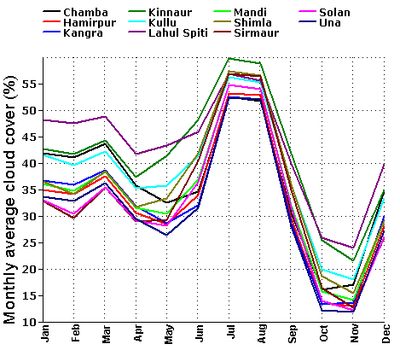
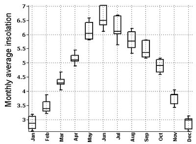
Cloud cover increases with increasing elevation as a consequence of the cloud-topography interactions and orographically-induced convection [32], evident from the monthly average cloud cover data procured from a 100 year meteorological dataset (Figure 6).  Lahul Spiti district in the high altitude alpine zone has the highest average cloud cover and solan district in the low altitude tropical zone has the least (Table 2). This also highlights the fluctuation in cloud amount over the advection facing and opposite sides of the mountains [32]. The relief elevation of the region and the resultant cloud cover influences the regional variation in insolation to a bigger extent even while considering the seasonal influences. These variations in insolation are apparent in the box plots given in figures 7, 8 and 9. The insolation in Himachal Pradesh is observed to increase from high altitude cold and dry alpine zone to the low altitude warmer tropical regions (below 1000 m). This regional variation in the magnitude of insolation is seen for a major part of the year from November to June while the trend reverses during July to October, with the high altitude zone receiving comparatively higher insolation. This could be attributed to the Southwest monsoon and the increase in cloud cover over the low as well as middle altitude regions (below 3500m) and the northeast dry monsoon winds from Central Asia setting in October.

Table 2: Regional variations, monthly average and standard deviations of global insolation

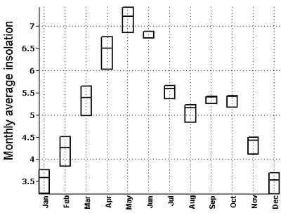
Figure 6: District wise monthly average cloud cover (%)

It has already been noted that March to October is a favourable period when the state receives good incident solar energy. In November, while low and middle altitude districts of Una, Bilaspur, Hamirpur, Kangra, Solan, Sirmaur, Mandi, Chamba and Shimla (below 3500m) enjoy insolation above 4 kWh/m²/day, the high altitude districts of Kullu, Lahaul Spiti and Kinnaur receive insolation below that. December and January witness the least insolation values in Himachal Pradesh with a maximum of ~3.75 kWh/m²/day even in the potential low altitude districts of the hill state. While the low and middle altitude districts pick up with increasing magnitude of insolation towards the end of January, the higher regions continue receiving lower insolation till the end of February. The low as well as middle altitude districts receive the highest average insolation above 7 kWh/m²/day in the month of May. In the case of high altitude districts, the highest insolation is observed in the month of June with an average of ~6.60 kWh/m²/day. Solar potential contours were developed based on the spatial distribution to explore the regional variations, and are illustrated in Figures 10 and 11 respectively. The global insolation spatial data indicate the monthly variations in insolation over the diverse topography of Western Himalayas. These variations could be attributed to the influence of the season, elevation and orography.

Table 3: Solar radiation data through ground based pyranometer [2]

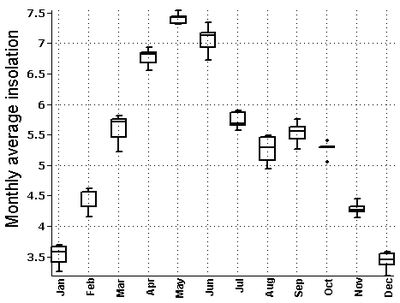
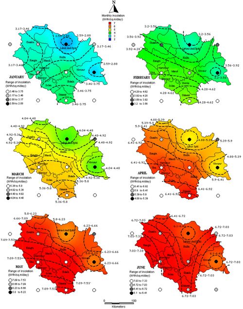
Figure 7: Variation of monthly average insolation in high altitude (above 3500 m) regions

Figure 8: Variation of monthly average insolation in middle altitude (1000-3500m) regions

Figure 9: Variation of monthly average insolation in low altitude (below 1000m) regions

Validation with ground data

Spatial variation of Global insolation  with the regional variation contours for the months of January – June is given in Figure 10, while Figure 11  presents the variation during July-December.  These  were validated with the monthly Global insolation data based on pyranometric data from ground radiation stations  [2], given in table 3 (RMSE of 4.88%).

Figure 10: Spatial variation of Global insolation  with the regional variation contours for the months of January - June

Figure 11: Spatial variation of Global insolation  with the regional variation contours for the months of of July – December

Conclusion

Spatial analysis of global insolation data aided in identifying the localities suitable for implementation of solar technologies. Satellite derived datasets available in user friendly formats based on time tested and realistic models provide solar radiation data on higher spatial and temporal scales, evident from the current endevour based on the 22 year average monthly global insolation data obtained from NASA SSE datasets. Solar potential of Himachal Pradesh was mapped and validated with the ground data obtained from radiation stations in India. The study demonstrates that the hill state receives global insolation (above 4 kWh/m²/day during the period of March to October) favourable for commercial solar applications.  The low and middle altitude regions (below 3500vm) receive similar global insolation during the months of February and November as well. The low and middle altitude regions receive similar Global insolation during the months of February and November as well. The state witness low average insolation values in the cold months of December and January mostly favouring domestic solar appliances like solar cooker, solar water heater etc. The solar maps obtained help in the design of appropriate solar energy devices for Himachal Pradesh which is facing ecological disasters in the wake of depleting resources. Conspicuously, they also provide suitable information for areas like meteorology, agriculture, forestry etc. This regional level understanding of solar potential will aid the policy makers, entrepreneurs as well as researchers especially in the context of the National Solar Mission of the Government of India.

Acknowledgement

 We thank NASA for making available the SSE datasets for renewable energy potential assessment throughout the world. The India Water Portal provides 100 years district wise meteorological data for India.  We are grateful to NRDMS  division, the Ministry of Science and Technology, Government of India and Indian Institute of Science for the financial and infrastructure support.

References

1. Kishore V V N, Renewable Energy Engineering and Technology : A knowledge compendium , TERI Press, New Delhi, 2008
2. Mani A., Handbook of solar radiation, Allied Publishers, New Delhi, 1981
3. World Meteorological Organisation, Viewed on July 29 2010, <http://www.wmo.int/pages/prog/arep/gaw/solar-radiation.html>
4. Varshita R D and Gupta M K, Modernisation of Radiation Network, Indian Meteorological Department, Pune, India, Viewed July 29 2010, <http://www.wmo.int/pages/prog/www/IMOP/publications/IOM-82-TECO_2005/Posters/P1%2810%29_India_Vashistha.pdf>
5. NASA, Surface Meteorology and Solar Energy Release 6.0 Methodology,  Viewed 29 July 2010, <http://eosweb.larc.nasa.gov/sse/documents/SSE6Methodology.pdf>
6. Alberto Ortega, Rodrigo Escobar, Sergio Colle, Samuel Lunade Abreu, The state of solar energy resource assessment in Chile, Renewable energy, 35, (2010) 2514 – 2524
7. Gayathri Vijayakumar, Michael Kummert, Sanford William A. Beckman, Analysis of short-term solar radiation, Solar Energy, 79, (2005) 495–504
8. Pitz-Paal, R, Geuder Norbert, Hoyer-Klick Carsten, Schillings Christoph, 2007, How to get bankable meteodata ? DLR solar resource assessment, NREL 2007 parabolic trough technology workshop, Golden, Colorado, Viewed August 1 2010, <http://www.nrel.gov/csp/troughnet/pdfs/2007/pitz_paal_dlr_solar_resource_assessment.pdf >
9. Ramachandra T V and Subramanian D K, Potential and prospects of solar energy in Uttara Kannada district of Karnataka State, Energy Sources, 19, (1996) 945 – 988 
10. Kun Yang, Toshio Koike, Baisheng Ye, Improving estimation of hourly, daily, and monthly radiation by importing global data sets, Agricultural and Forest Meteorology, 137, (2006) 43–55
11.  Xiaoying Liu, Xurong Mei, Yuzhong Li, Qingsuo Wang, Jens Rauns Jensen, Yanqing Zhang, John Roy Porter, Evaluation of temperature-based global solar radiation models in China. Agricultural and Forest Meteorology, 149, (2009) 1433–1446
12. Liu D.L. and Scott B.J., Estimation of solar radiation in Australia from rainfall and temperature observations, Agricultural and Forest Meteorology, 106, (2001) 41–59
13.  Jimmy S G, Ehnberg, H.J. Math, Simulation of global solar radiation based on cloud observations, Solar Energy, 78, (2005) 157–162
14.  Ramachandra T V, Solar energy potential assessment using GIS, Energy Education Science and Technology, 18, Issue 2, (2007) 101-114
15. Adnan Sozen, Erol Arcaklioglu, Solar potential in Turkey, Applied Energy, 80, (2005) 35 – 45
16. Kishtawal C.M., Meteorological Satellites, Satellite Remote Sensing and GIS Applications in Agricultural Meteorology, pp. 67-79, viewed August 1 2010 <http://www.wamis.org/agm/pubs/agm8/Paper-4.pdf>
17. Malik A.Q., Mufti A., Hiser H.W., Veziroglu N.T.and  Kazi L., Application of Geostationary data for determining solar radiation over Pakistan, Renewable Energy, 1, (1991) 455-461
18. John E Hay, Satellite based estimates of solar irradiance at the earth's surface - I Modelling approaches, Renewable energy, 3, (1993) 381- 393
19. Chumnong Sorapipatana, An assessment of solar energy potential in Kampuchea, Renewable and Sustainable Energy Reviews, 14, (2010) 2174–2178
20. Frulla L.A., Grossi Gallegos, Gagliardini T.D.A. and Atmnzai G., Analysis of satellite measured insolation in Brazil, Solar & Wind Technology, 7, (1990) 501-509
21.  Tanahashi S.,  Kawamura H.,  Matsuura T., Takahashi T, and  Yusa H., Improved estimates of hourly insolation from GMS S-VISSR data, Remote sensing of environment, 74, (2000) 409 – 413
22.  Cogliani E., Ricchiazzi P. and Maccari A., Generation of operational maps of global solar irradiation on horizontal plan and of direct normal irradiation from meteosat imagery by using SOLARMET, Solar energy, 82, (2008) 556 – 562
23.  Janjai S.,  Pankaew P. and Laksanaboonsong J., A model for calculating hourly global solar radiation from satellite data, Applied Energy, 86, (2009) 1450 – 1457
24. Islam M.D., Alili A.A., Kubo I and  Ohadi M., Measurement of solar-energy (direct beam radiation) in Abu Dhabi, UAE, Renewable Energy, 35, (2010) 515–519
25. Richard Perez, Robert Seals, Antoine Zelenka, Comparing satellite remote sensing and ground network measurements for the production of site/time specific irradiance data,  Solar Energy, f50, (1997) 89-96
26. Illera P., Fernfindez A, and Perez A., A simple model for the calculation of global solar radiation using geostationary satellite data, Atmospheric Research, 39, (1995) 79 – 90
27. Statistical Data of Himachal Pradesh upto 2009-10, Himachal Pradesh Planning Department, Govt. of Himachal Pradesh, Viewed on August 2, 2010, <http://hpplanning.nic.in/Statistical data of Himachal Pradesh upto 2009-10.pdf>
28. SRB Data and Information, Atmospheric Science Data Center, NASA, Viewed August 2, 2010 <http://eosweb.larc.nasa.gov/PRODOCS/srb/table_srb.html>
29. NASA/GEWEX Surface Radiation Budget Project, Viewed August 2 2010, <http://gewex-srb.larc.nasa.gov/>
30. Gupta S.K., Wilber A.C., Kratz D.P. aand Stackhouse Jr. P.W., The Langley Parameterized Shortwave Algorithm (LPSA) for Surface Radiation Budget Studies, NASA/TP-2001-211272, 2001
31. Gupta S.K., Whitlock C.H., Ritchey N.A. and Wilber A.C., An Algorithm for Longwave Surface Radiation Budget for Total Skies, CERES ATBD Subsystem 4.6.3 , Viewed August 2 2010,   http://ceres.larc.nasa.gov/documents/ATBD/pdf/r2_2/ceres-atbd2.2-s4.6.3.pdf
32. Andrzej Z. Kotarba, Satellite-derived cloud climatorlogy over high elevation areas based on circulation types: A 2007 analysis of the Tatra Mountains, Physics and chemistry of the earth, 35, (2010) 462 – 468

BACK  «  TOP  »  NEXT