| CES Technical Report 131, August 2013 |
|
Ecological Modelling and Energy DSS |
|
Above Ground Standing Biomass of three micro watersheds in Himachal Pradesh |
|
Introduction
Biomass in all its form provides about 14% of the world’s energy (Hall and Challe, 1991). The dependency on forest resources is high in developing countries like India, which has an estimated 329 million hectares that can be used for biomass production under various classes like cropland, forests, plantation, etc. The projected biomass demand for India is around 516 Mt/yr (Bhattacharya et al. 2003).
Forests play an important role in global carbon cycling, since they are large pools of carbon as well as potential carbon sinks and sources to the atmosphere. Accurate estimation of forest biomass is required for greenhouse gas inventories and terrestrial carbon accounting. The needs for reporting carbon stocks and stock changes for the Kyoto Protocol have placed additional demands for accurate surveying methods that are verifiable, specific in time and space, and that cover large areas at acceptable cost (IPCC, 2003; Krankina et al. 2004; Patenaude et al. 2005; UNFCCC, 1997).
Forest biomass varies over climatic zone, altitude and region (Brown et al., 1989). Plant biomass is therefore a metric fundamental to understanding and managing forest ecosystems, whether to estimate primary production, nutrient pools, species dominance, responses to experimental manipulation, or fuel loads for fire. In recognition of its central importance, models of ecosystem processes often include plant biomass or biomass-related variables as inputs and outputs (Northup et al. 2005).
In the Himalaya, vegetation ranges from tropical monsoon forest to alpine meadow and scrub, across elevation gradients. The Himalayan forest biomass is important as a large population of hill folk are still dependent on forest biomass to meet their daily requirement (Singh and Singh, 1987). The trend in biomass in the Himalayan region shows an increase in biomass with increase in altitude for different strands up to an altitude of 2700 m and shows decrease hence on, as the vegetation above 3000 m is sparse and are mostly of alpine grassland types at above 3500 m (Singh et al. 1994)
Pinus roxburghii Sarg. (chir pine) forest are dominant along the low-to-mid montane belt of Central and Western Himalaya (Chaturvedi and Singh, 1987) due to high regeneration potential, growth rate, establishing in degraded habitats, pipe like boles and high volumes.
Disturbance has become a widespread feature in most of the forests all over the Himalaya (Singh and Singh, 1992), therefore, knowledge on ecological processes and biotic pressure can help in understanding the persistence of long-lived plant communities. A sustained regeneration and growth of all species in the presence of older plants is required for better growth of any plant community (Ramakrishnan et al., 1981). Humans have made considerable impacts in the Himalayan region, estimating such changes accurately would be of particular value to Himalayan people, whose subsistence agriculture depends on forest productivity to maintain livestock and soil fertility.
For an assessment of forest biomass, forest inventory is most commonly used and it differs depending on scope and purpose. Inventories are being designed to obtain information on other uses of the forest like recreation, grazing, wildlife and water conservation. It is designed to measure forest biomass rather than or in addition to traditional volume. Species specific equations that describe relationships between plant attributes and biomass are more accurate and flexible. Furthermore, it is preferable to use region or site-specific relationships where possible. Species size–biomass relationships could differ as plants alter allocation patterns in response to soils, climate and disturbance. Changes in structure and composition of vegetation are often accompanied by changes in biomass. (Brown and Luo 1992). Forest biomass varies over climatic zone, altitude and region (Brown et al., 1989, 1991)
In this report we have examined the variation in above ground standing biomass of three micro watersheds which has a forest widely used by the local people for fuel wood, fodder, and for grazing of cattle in the Himachal Pradesh region across varying altitude and vegetation types.
Methods
Study Area:
The department of Science and Technology (DST), Government of India, has taken a major initiative to create a bio-geo database and ecological modelling for western Himalayas. Initially three watersheds have been identified in Himachal Pradesh. The three micro watersheds having typical mountain village ecosystem were selected across three altitudinal zones (Figure 1). The forests in the three watersheds are managed as reserve forest by the state forest department, where cutting of trees is prohibited. However, lopping and collection of fallen wood for household purpose by the villagers are noted in all three watersheds. Spatial bounds of the respective watersheds were delineated from the digital elevation model (DEM) generated from the remote sensing data. The characteristics of the watersheds is summarised in Table 1.
Table 1. Geographical attributes of study area
| Micro watersheds |
District |
Main watershed |
Latitude (°N) |
Longitude (°E) |
Altitude(m amsl) |
Area (sq.km) |
| Mandhala |
Solan |
Yamuna |
30.87-30.97 |
76.82-76.92 |
400-1100 |
14.53 |
| Moolbari |
Shimla |
Yamuna |
31.07-31.17 |
77.05-77.15 |
1400-2000 |
10.50 |
| MeGad |
Lahaul and Spiti |
Chandrabhaga |
32.64-32.74 |
76.46-76.74 |
2900-4500 |
46.05 |

Figure 1: Boundary map of three watersheds
* - indicates the location of villages in the watershed
Climate
The climate is distinguished in three axes, in the Western Himalayas: (1) a vertical axis determined by the effect of altitude on temperature; (2) a transverse axis determined by topography along which rain shadow effects cause decreasing precipitation and increasingly extreme (continental) temperature fluctuations from SW to NE across the main ranges; (3) a longitudinal axis determined by a geographical trend of decreasing monsoon precipitation (June-September) and increasing winter snowfall (December-April) from SW to NW along all the ranges. The third axis is important in determining major ecological trends over the entire length of the Himalayan chain, but it is less important than the other two axes in determining the ecology of localities within the Western Himalayas (Gaston et al., 1983).
Vegetation type
The three watersheds represent different vegetation types;
Mandhala watershed: This watershed falls in lower shiwalik range (400 - 1100m) and are characterised by dry evergreen tree species and scrub vegetation. The major tree species in this watershed is Flacourtia montana, Acacia catechu, Grewia optiva, Toona ciliata, Albizia procera, Haldina cordifolia, Acacia sp., Lannea coramandelica, Mitragyma parviflora, along with Nyctanthus arbor-tristis, Carissa apaca, Dodonaea viscose and Woodfordia fruticosa. Most of the forests here have been deforested and hill ranges completely covered with Lantana camera weed. Also scattered trees of Holoptelia integrifolia, Dalbergia sisoo, Morus nigra, etc. occur along the field bunds and other open lands.
Moolbari watershed: The vegetation here is characteristically of middle temperate type of the Himalayan region of the mid altitude ranges (1400-2000m). The vegetation in this watershed consisted of mixed deciduous and sub-tropical pine forest in two different altitudinal ranges. Former till an altitude of 1500m and later beyond 1500m. Apart from Pinus other species seen are Pyrus pashia, Rubus ellipticus, Berberis sp, and in moist localities species of Quercus leucotrichophora and Q. glauca and Rhododendron arboretum. On the exposed hill slopes in pine forests Euphorbia royleana is encountered. Between 1800-2000 m, oak forests species such as Quercus leucotrichophora, Q. glauca dominate along with Rhododendron arboretum, Lyonia ovalifolia.
MeGad Watershed: This watershed falls in the rain shadow region of the Himalayas (2900-4500m), and receives less than 80cm rainfall annually, there is high snowfall during winter and temperature goes to as low as -20˚C in this season. This watershed comprises of temperate, alpine and sub-alpine vegetation.
- Temperate vegetation: It consists of woody trees at altitude of 2500-3200 such as Pinus wallichiana, Juniperus recurva, Picea smithiana, Abies pindrow, Cedrus deodara that form the natural forests. Along the streams and irrigated canals are planted trees of Salix and Popular sp.
- Alpine - Sub-alpine vegetation: Mostly stunted, scattered bushes of Juniperus communis, Berberis sp., etc along with herbaceous elements such as Ranunculus, Pedicularis, Potentilla, Polygonum, Geranium, Anemone, Corydalis, etc., are commonly encountered.
Quantification of Bioresources
Vegetation Sampling to estimate Above Ground Biomass (AGB)
Belt transect of 250 x 4 m was laid randomly throughout the water shed. In each transect, for each tree GBH (Girth at Breast Height in cm) and height (in m) is noted along with its identification. Coordinates were marked using GPS at the start and end points in each transect and at every 100m interval. Litter weight is measured in four 1m X 1m quadrat within each transect. Using densiometer, canopy cover is measured at start, end point and at 100 meter interval in each transect.
The above ground standing biomass is estimated transect wise through non-destructive sampling using standard regression models suitable for these agro-climatic zones (Brown et al., 1989; Schroeder et al., 1997) and are given in Table 2. The AGB is estimated for each transect in all three watersheds and represented as tonnes/hectare (t/ha).
Table 2. Regression models used to estimate AGB in the study region
| Regression model |
Study region |
Model # |
| AGB = exp{-1.996+2.32*ln(D)} |
Mandhala, MeGad |
1 |
| AGB = 10^{-0.535+Log10 (BA)} |
Mandhala, MeGad |
2 |
| AGB = 42.69-12.800(D)+1.242(D2) |
Moolbari |
3 |
| AGB = exp{-2.134+2.530*ln(D)} |
Moolbari |
4 |
| AGB= (0.5+25000D2.5)/(D 2.5+246872) |
Moolbari |
5 |
Note: AGB=Above ground biomass (t/ha), D=diameter at breast height (cm), BA =Basal Area (sq.cm)
Results
AGB in Mandhala
Mandhala watershed falls in the lower Shiwaliks, receives low rainfall and hence are considered as dry regions. We used Model 1 and 2 from Table 2 for estimation of AGB. Table 3 provides transect-wise estimated AGB in Mandhala watershed.
Table 3. Transect-wise AGB in Mandhala watershed
| Transect # |
Basal Area (sq.cm) |
Model 1 (t/ha) |
Model 2 (t/ha) |
| 1 |
5969.9 |
31.60 |
17.42 |
| 2 |
12398.1 |
69.80 |
36.17 |
| 3 |
8993.1 |
44.79 |
26.24 |
| 4 |
4060.3 |
17.91 |
11.85 |
| 5 |
5386.4 |
33.02 |
15.71 |
| 6 |
5697.4 |
21.66 |
16.62 |
| 7 |
685.0 |
2.71 |
2.00 |
| 8 |
4317.8 |
15.18 |
12.60 |
| 9 |
4862.5 |
21.70 |
14.19 |
| 10 |
2084.4 |
8.92 |
6.08 |
| 11 |
2615.4 |
12.58 |
7.63 |
| Mean±Sd |
5188.23±256.32 |
25.44±18.93 |
15.14±9.5 |
| Range |
685.0 - 12398.1 |
2.71 - 69.8 |
2.00 - 36.17 |
Estimated AGB varied from 2.71-69.8 to 2.00-36.17 t/ha according to respective models. The variations among transects were significantly different (Analysis of Variance, ANOVA, F = 3.97, P=0.04) between Model 1 and 2, though the overall estimate is not different between the models (Students t, t=1.61, P=0.12). Figure 2 is the scatter plot of basal area against above ground biomass estimate based on Model 1 and Model 2. Model 2 mentioned in Table 4 is better suited for Mandhala water shed (n=11, R2=1).
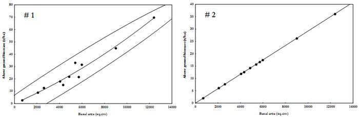
Figure 3. Scatter plot for AGB estimation in Mandhala watershed.
Table 4. AGB estimation regression models based on basal area (BA in sq.cm).
| Model # |
Regression model |
R2 |
| 1 |
AGB=0.0497+0.004(BA)+1E-7(BA2) |
0.97 |
| 2 |
AGB=0.0012+0.0029(BA) |
1.0 |
AGB in Moolbari
This watershed falls in mid Himalayan ranges and receives higher rainfall (compared to Mandhala and MeGad). Regression models 3, 4 and 5 for wet region are used to estimate AGB. Table 5 provides transect-wise estimated AGB in Moolbari watershed.
Table 5. Transect-wise AGB in Moolbari watershed.
| Transect # |
Basal area (sq.cm) |
Model 3 (t/ha) |
Model 4 (t/ha) |
Model 5 (t/ha) |
| 1 |
25101.27 |
274.56 |
246.86 |
246.86 |
| 2 |
16690.37 |
157.52 |
134.48 |
102.58 |
| 3 |
14587.18 |
127.35 |
107.89 |
83.21 |
| 4 |
11312.74 |
87.26 |
75.88 |
58.90 |
| 5 |
13514.97 |
123.86 |
104.94 |
80.45 |
| 6 |
32371.50 |
285.80 |
240.78 |
185.81 |
| 7 |
26968.07 |
236.72 |
202.23 |
155.51 |
| 8 |
28952.87 |
205.99 |
182.35 |
142.79 |
| 9 |
7301.27 |
54.92 |
47.26 |
36.99 |
| 10 |
34736.07 |
261.03 |
228.06 |
177.72 |
| 11 |
31389.01 |
254.35 |
230.21 |
174.21 |
| 12 |
30605.41 |
280.61 |
242.64 |
184.45 |
| 13 |
22370.38 |
191.97 |
166.93 |
127.96 |
| 14 |
23891.16 |
199.65 |
175.47 |
134.37 |
| 15 |
23362.76 |
195.78 |
166.74 |
129.26 |
| 16 |
24085.99 |
191.40 |
166.70 |
129.16 |
| Mean±Sd |
22952.56±8146.31 |
195.55±70.22 |
169.96±62.03 |
134.39±53.91 |
| Range |
7301.27-34736.07 |
54.92 – 285.80 |
47.26-246.86 |
36.99-246.86 |
Variations among transects were not significant (Model 3 vs. 4, F=1.28, p=0.64; Model 3 vs. 5, F=1.7, p=0.32; and Model 4 vs. 5, F=1.32, p=0.59), indicating homogeneity among transects. Among the three models, mean AGB estimate between models were also similar, except for model 3 and 5 (Model 3 vs. 4, t=1.09, p=0.28; Model 4 vs. 5, t=1.73, p=0.094; and Model 3 vs. 4, t=2.76, p=0.009). Figure 3 is the scatter plot of basal area against above ground biomass estimate based on Models 3, 4 and 5. Table 6 lists the models with their R2 values.
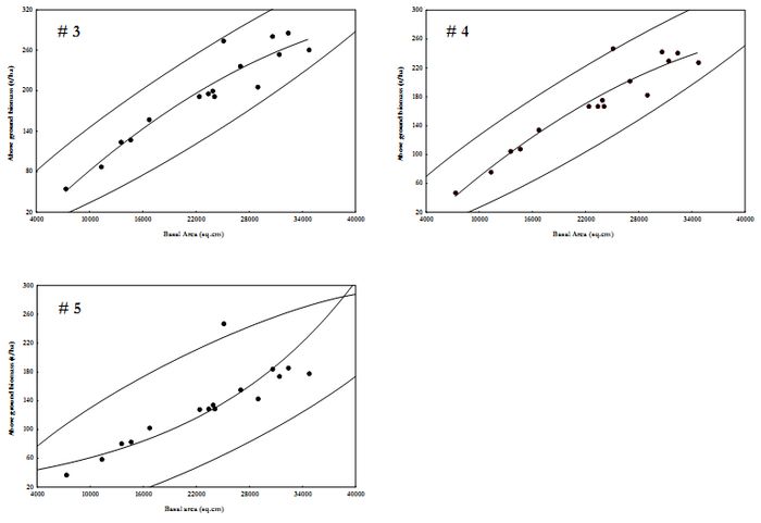
Figure 4. Scatter plot for AGB estimation in Moolbari watershed.
Table 6. AGB estimation regression models based on basal area (BA in sq.cm, n=16).
| Model # |
Regression model |
R2 |
| 3 |
AGB=-42.176+0.014(BA)-1.3E-7(BA2) |
0.91 |
| 4 |
AGB=-39.984+0.0121(BA) -1.0E-7(BA2) |
0.90 |
| 5 |
AGB=35.596e5.0E-5(BA) |
0.82 |
AGB was also estimated considering entire Moolbari watershed as temperate broadleaf forest and dividing further according to dominant forest type (Table 7).
Table 7. Species-wise estimate of AGB in Moolbari watershed.
| Forest type |
Model |
AGB (t/ha) |
Reference |
| Quercus forest |
AGB = 1.8409BA 0.89262 |
221.79 |
Li and Luo (1996) |
| Pine and other conifers |
AGB= 0.5168*(Volume)+33.2378 |
31.26 |
Fang et al., (1998) |
| Miscellaneous broad leaved |
AGB=0.5+25000D 2.5 /D 2.5+ 246872 |
19.17 |
Schroeder et al., (1997) |
| Total |
|
272.22 |
|
AGB in MeGad Watershed
For the marked reduction in precipitation, MeGad is considered as dry region for the estimation of AGB. Table 8 details the estimated AGB based on Model 1 and 2 listed in Table 2.
Table 8. Transect-wise AGB in MeGad watershed.
| Transect # |
Basal Area (sq.cm) |
Model 1 (t/ha) |
Model 2 (t/ha) |
| 1 |
20513.61 |
112.70 |
59.85 |
| 2 |
23629.62 |
135.45 |
68.94 |
| 3 |
35090.13 |
221.44 |
102.37 |
| 4 |
19964.49 |
114.94 |
58.25 |
| 5 |
2067.44 |
9.06 |
6.03 |
| 6 |
25217.91 |
161.56 |
73.57 |
| 7 |
40590.37 |
248.65 |
118.42 |
| Mean±Sd |
23867.65±12309.93 |
143.4±78.91 |
69.63±35.91 |
| Range |
2067.44-40590.37 |
9.06-248.65 |
6.03-118.42 |
On comparing Model 1 vs. Model 2, mean estimate of AGB were significantly different (t=2.25, P=0.044). AGB estimates for each transect varied considerably, although not statistically significant (F=4.83, P=0.08). Figure 4 depicts basal area against AGB in MeGad watershed and regression models of the same are in Table 9.
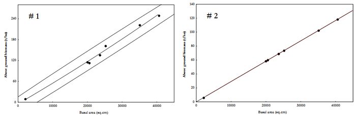
Figure 5. Scatter plot for AGB estimation in MeGad watershed.
Table 9. AGB estimation regression models based on basal area (BA in sq.cm).
| Model # |
Regression model |
R2 |
| 1 |
AGB=-4.4259+0.0058(BA)+1E-8(BA2) |
0.99 |
| 2 |
AGB=0.0013+0.0029(BA) |
1.0 |
Both model 1 and 2 have significant r2 values. Model 2 is better suited than model 1 for its simplicity in calculation. Considering different forest types, AGB estimated for MeGad are listed in Table 10. These estimates vary from 140.37 to 400.34t/ha for the region.
Table 10. Species-wise estimate of AGB in MeGad watershed.
| Forest type |
Model |
AGB (t/ha) |
Reference |
| Picea - Abies forest |
AGB = 50.8634 + 0.5406(BA) |
400.34 |
Li and Luo (1996) |
| Mixedconifers |
AGB= 0.5168*(Volume)+33.2378 |
352.93 |
Fang et al., (1998) |
| Pines and other conifers |
AGB= 0.5168*(Volume)+33.2378 |
336.96 |
Fang et al., (1998) |
| Conifers |
AGB= (0.5+15000D 2.7) /(D 2.7+ 364946) |
140.37 |
Schroeder et al., (1997) |
Validation of Biomass results:
The results of biomass estimation for the three watersheds were validated with the biomass estimation results in published literature.
| Altitude range |
Biomass range
(Observed) |
Biomass obtained |
| Quercus |
200-550 |
221.79 |
| Abies- pindrow |
52-512 |
400.34 |
| Pine forest |
28-365 |
336.96 |
Evergreen broad leaved
Quercus forest |
46-72734-516 |
19.17221.79 |
| Dry evergreen forest type |
39-170 |
25.14 |
The results show that for most of the forest types in the study area, the biomass obtained is well within the range of biomass obtained in similar forests. However very low biomass is noted in Mandhala watershed, the forests of Mandhala region are highly degraded and invasive weeds like lantana and euphotorium have put constraint on the growth and regeneration of natural vegetation
Litter Weight:
The dry litter in the ground is measured in each belt transect at start point, end point and at every hundred metre interval. A plot of 1m X 1m is made and all the dry leaf litter falling within the plot is collected in a bag and weighed with a 500g spring balance.
Table 9: Values of Litter weight and canopy cover in transects
| Litter weight in grams |
Canopy cover in % |
Litter wt |
Canopy cover closed |
| 90 |
32.4 |
110 |
36 |
| 80 |
52.16 |
370 |
76 |
| 10 |
0 |
70 |
74 |
| 120 |
53.2 |
170 |
82 |
| 45 |
11.6 |
130 |
92 |
| 130 |
91.68 |
120 |
56 |
| 20 |
0.16 |
80 |
54 |
| 40 |
25.12 |
90 |
35 |
| 170 |
81.28 |
125 |
4 |
| 370 |
75.04 |
0 |
8 |
| 120 |
4.32 |
350 |
72 |
| 110 |
33.44 |
0 |
2 |
| 80 |
29.28 |
250 |
76 |
| 150 |
81.28 |
0 |
4 |
| 260 |
92.72 |
270 |
96 |
| 240 |
91.68 |
0 |
5 |
| 310 |
41.76 |
0 |
4 |
| 70 |
72.96 |
|
|
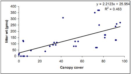
Graph 1: Litter Weight and canopy cover
A graph was plotted between the litter weight and canopy cover. A linear trend line was plotted in the graph to see the relation; though not much a significant relation is seen, increase in canopy cover will cause the litter weight to increase.
Discussion
In the Himalaya, vegetation ranges from sub-tropical monsoon forest to alpine meadow and scrub, across elevation gradients. Plant species richness in the three watersheds varied along elevation and is represented in Figure 6. The overall trend indicates a gradual increase in species richness till mid altitudinal regions and then decrease with increase in elevation. Though the polynomial relationship is not significant (r2=0.32), but this is similar to general pattern of species richness along elevation in the Himalayas. Such pattern is evident in relative abundance of plant species.
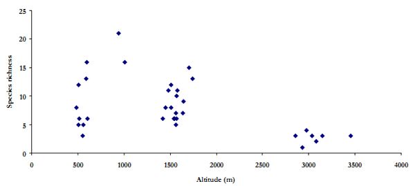
Figure 6. Plant species richness along elevation gradient in the three watersheds.
Figure 7 illustrates the trend in relative abundance (no. of individuals/1000 sq.m) of plant species in each transect against elevation gradient. It is interesting to note that, low altitude (500-1000m) and very high altitude (2700-3500m) had lesser abundance compared to mid altitude (1300-1600m).
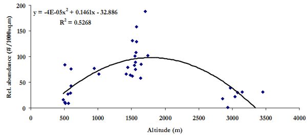
Figure 7. Relative abundance along elevation gradient in the three watersheds.
Species richness has not influenced the relative abundance in the three watersheds as evident in Figure 8 (r2=0.26). Hence, it can be inferred here that relative abundance of the individuals in a region influences the AGB than species richness. This apparent non-influence is evident in scatter plot of species richness against AGB (Figure 9, r2=0.005 ).
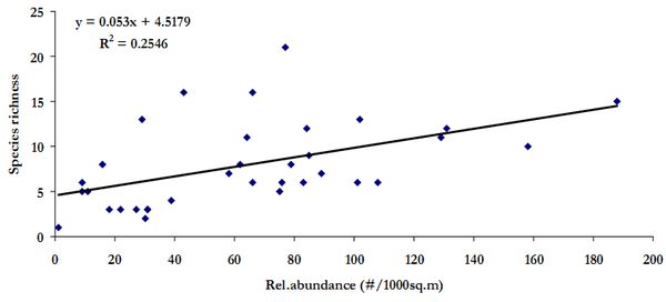
Figure 8. Scatter plot of relative abundance versus species richness in three watersheds
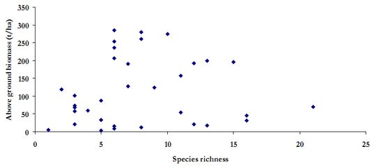
Figure 9. Scatter plot of species richness and above ground biomass in the study region
Influence of relative abundance on the AGB estimate in the study region is illustrated in Figure 9. The apparent lower AGB estimate at higher abundance are due to plantation trees of lower girth classes from Mandhala water shed.
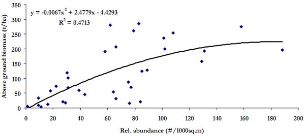
Figure 10. Scatter plot of relative abundance and above ground biomass in the study region
The trend in biomass in the Himalayan region shows an increase in biomass with increase in altitude for different strands up to an altitude of 2700 m and shows decrease hence on, as the vegetation above 3000 m is sparse and are mostly of alpine grassland types at above 3500 m (Singh et al. 1994). This is evident in Figure 10 based on elevation gradient and estimated AGB in the study area.
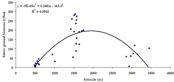
Figure 11. Scatter plot of above ground biomass against elevation gradient
Pinus roxburghii Sarg. (chir pine) forest are dominant along the low-to-mid montane belt of Central and Western Himalaya (Chaturvedi and Singh, 1987) due to high regeneration potential, growth rate, establishing in degraded habitats, pipe like boles and high volumes.
Disturbance has become a widespread feature in most of the forests all over the Himalaya (Singh and Singh, 1992), therefore, knowledge on ecological processes and biotic pressure can help in understanding the persistence of long-lived plant communities. A sustained regeneration and growth of all species in the presence of older plants is required for better growth of any plant community (Ramakrishnan et al., 1981). Humans have made considerable impacts in the Himalayan region, estimating such changes accurately would be of particular value to Himalayan people, whose subsistence agriculture depends on forest productivity to maintain livestock and soil fertility.
The distribution and dynamics of biological resources must be understood to provide a rational basis for planning and management decisions, without which conservation of these resources in the natural habitats would be impossible (Keith and Sanders, 1990; Khoshoo, 1992).
Land use patterns needs to be considered before analyzing the area that will be potentially available for biomass production, it is essential to understand the projected trends in land use pattern for the future.
Watershed approach in the Himalayan region has become acceptable in undertaking land improvement measures (Sharma et al.1992), however, the development has not achieved the desired pace due to lack of information available on the watershed level and because of sectoral approaches adopted by various departments working in the Himalaya (Sundriyal et al. 1994b).
Therefore, in many areas re-construction of disturbed ecosystems should be taken up on a priority basis, both for biodiversity conservation and for maintaining landscape productivity (Behera et al., 2006)
Conclusion
The basal area, tree density and biomass per hectare is high for the watershed in the middle elevation, the mid domain effect observed in the Himalayan region is same here. The basal area and number of trees/ha for all three watershed is less than in comparison with undisturbed sites of the Himalayan region.
References:
- Aboal, J. R.; Arevalo, J. R. & Fernandez, A. (2005), 'Allometric relationships of different tree species and stand above ground biomass in the Gomera laurel forest (Canary Islands)', Flora - Morphology, Distribution, Functional Ecology of Plants 200(3), 264--274.
- Behera S K., Misra M.K. 2006. Above ground biomass in a recovering tropical sal (Shorea robusta Gaertn.f.) forest of Eastern Ghats, India. Biomass and Bioenergy 30 :509–521
- Bhat D.M, Ravindranath N.H, Gadgil M, 1995, Effect of Lopping intensity on tree growth and stand productivity in tropical forest. Journal of Tropical Forest Science 8(1): 15-23
- Bhattacharya, S. C.; Salam, P. A.; Pham, H. L. & Ravindranath, N. H. (2003), 'Sustainable biomass production for energy in selected Asian countries', Biomass and Bioenergy 25(5), 471--482.
- Brown, S., 1997. Estimating biomass and biomass change of tropical forests. A primer. FAO Forestry Paper 134. Food and Agriculture Organization of the United Nations, Rome, Italy.
- Brown Sandra, Schroeder Paul, Birdsey Richard. 1997. Aboveground biomass distribution of US eastern hardwood forests and the use of large trees as an indicator of forest development, Forest Ecology and Management. 96:37-47.
- Brown Sandra., Schroeder Paul, Kern Jeffrey S. 1999. Spatial distribution of biomass in forests of the eastern USA, Forest Ecology and Management. 123: 81-90
- Brown, S and A.E. Lugo, 1990. Tropical secondary forests, J. Trop. Ecol. 1990: 1–32
- Chave, C. Andalo, S.L. Brown, M.A. Cairns, J.Q. Chambers, D. Eamus, H. Fölster, F. Fromard, N. Higuchi, T. Kira, J.P. Lescure, B.W. Nelson, H. Ogawa, H. Puig, B. Riéra and T. Yamakura, Tree allometry and improved estimation of carbon stocks and balance in tropical forests, Oecologia 145 (2005), pp. 87–99.
- Chaturvedi O.P and Singh J.S, 1987, The Structure and Function of Pine Forest in Central Himalaya. I. Dry Matter Dynamic, Annals of Botany 60: 237-252
- Fang J Y, GG Wang, GH Liu, SL Xu,1998, Forest Biomass of China: An Estimate Based on the Biomass-Volume Relationship, Ecological Applications,8(4) pp 1084-1089
- Garkoti S.C, Singh S.P, Variations in the Net primary productivity and Biomass of forests in high altitude region in the central Himalayan region. Journal of Vegetation Science, Vol 1, pp 23-28
- Gaston A.J, P.J Garson, M.L Hunter Jr, 1983, The status and conservation of forest Wildlife in Himachal Pradesh in Western Himalayas, Biological Conservation, 27 pp 291-314.
- IPCC 2003, Inter Governmental Panel on Climate Change, Report
- Keith D A and Sanders J.M, 1990, Vegetation of the eden region, south eastern Ausralia: Species composition diversity and Structure, Journal of Vegetation Science, Vol 1: 203-232
- Khoshoo, T.N., 1992. Plant Diversity in the Himalaya: Conservation and Utilization. G.B. Pant Memorial Lecture 1I, G.B. Pant Institute of Himalayan Environment and Development, Kosi, Almom-263443, 129 pp.
- Krankina Olga N, Mark E. Harmon, Warren B. Cohen ,Doug R. Oetter, Zyrina Olga and Maureen V. Duane, 2004, Carbon Stores, Sinks, and Sources in Forests of Northwestern Russia: Can We Reconcile Forest Inventories with Remote Sensing Results? Climate Change, Vol 67: No. 2-3, pp 257-272
- Luo tianxiang, Li wenhua, and Zhu huazhong. 2002. Estimated biomass and productivity of natural vegetation on the Tibetan plateau, Ecological Applications, 12:980–997
- Northup B.K., Zitzer S.F., Archer S., McMurtry C.R., Boutton T.W. 2005. Above-ground biomass and carbon and nitrogen content of woodyspecies in a subtropical thornscrub parkland. Journal of Arid Environments. 62: 23–43
- Schroeder, S. Brown, J. Mo, R. Birdsey and C. Cieszewski , Biomass estimation for temperate broadleaf forests of the US using inventory data. Forest Science 43 (1997), pp. 424–434
- Sharma.M, Current environmental problems and future perspectives, Tropical Ecology 37 (1996), pp. 15–20
- Sharrna, E., Sundriyal, R.C., Rai, S.C., Bhatt, Y.K., Rai, L.K., Sharma. R. and Rai, Y.K., 1992. Integrated watershed management: A case study in Sikkim Himalaya. Gyanodaya Prakashan. Nainital, 120 pp.
- Sundriyal, R.C., Sharma, E., Rai, L.K. and Rai, S.C., 1994a. Tree structure, regeneration and woody biomass removal in a subtropical forests of Mamaly watershed in the Sikkim Himalaya. Vegetation 113: 53-63.
- Patenaude G, R Milne, TP Dawson, 2005, Synthesis of remote sensing approaches for forest carbon estimation: reporting to the Kyoto Protocol, Environmental Science and Policy, Volume 8, Issue 2, pp 161-178
- Singh Arvind, Jha A.K. & Singh J.S. 1997. Influence of a developing tree canopy on the yield of Pennisetum pedicellatum sown on a mine spoil, Journal of Vegetation Science, 8:537-540.
- Singh Surendra P, Adhikari Bhupendra S., Zobel Donald B. 1994. Biomass, Productivity, Leaf Longevity, and Forest Structure in the Central Himalaya, Ecological Monographs, 64: 401-421.
- Singh Lalji and Singh J.S 1991, Species Structure, Dry Matter Dynamics and Carbon Flux of a Dry Tropical Forest in India, Annals of Botany 68: 263-273
- UNFCCC. 1997. “Climate Change Secretariat” [Web Page]. Available at http://www.unfccc.de/.
- UNFCCC. 1997. Kyoto Protocol to the United Nations Framework Convention on Climate Change. Kyoto: United Nations Framework Convention on Climate Change.
Annexure – I
Biomass is defined as the total amount of aboveground living organic matter in trees expressed as oven-dry tons per unit area. Biomass estimation of vegetation in general, forests in particular has received serious attention over the last few decades for the very reason that components of climate change are associated with change in the biomass of a region. From ecosystem perspectives, biomass estimation helps in ecosystem productivity, energy and nutrient flows, and for assessing the contribution of changes in forest lands to the global carbon cycle. The potential carbon emission that could be released to the atmosphere due to degradation of forest and forest resource, deforestation and conversion of forested area into other land-use can be determined by biomass estimation. Hence, the precise estimation of biomass becomes necessary for understanding the importance of forest both at global scale as well as regional scale for their impact in climate change.
Literature review
Methods involved in estimation of above ground biomass: There are two approaches for estimating aboveground biomass (AGB) in trees, namely
- Destructive,
- non-destructive.
The destructive method involves harvesting tree samples and estimating wood density and above ground biomass followed by deriving a probable relationship between tree girth, height with above ground biomass. Rai (1984) developed equations based on destructive sampling of four tropical rainforests of Western Ghats of Karnataka and compared the regression models against D2H and DBH (where D is diameter in cm, H is height in m and DBH is diameter at breast height in cm) , both in log and non-log models. Most of recent non-destructive methods involving allometric equations are based on earlier destructive sampling methods. Destructive sampling gives precise biomass estimation, but cannot be done in all situations and more over this requires considerable amount of trees to be cut. Hence biomass estimation through non-destructive method is adapted nowadays.
In non-destructive techniques, forest biomass is estimated mathematically, using functions which relate the diameter of a tree to its biomass- or parts of its biomass- (leaves, bark, bole wood etc). This approach is further divided into a direct approach using allometric equations, and an indirect approach using biomass expansion factors.
i) Allometry is the relation between the size of an organism and the size of any of its parts, and allometric equation is usually expressed in power-law form or in logarithmic form. Once an allometric equation has been developed, the biomass can be estimated in a forest stand using just the simple measurements of diameter.
The allometric equation's general form is usually written as,
y = bxa
or
ln y = lnb + aln x
where b is a constant, called allometric coefficient and a is the allometric exponent.
Ketterings et al. (2001) proposed allometric equation based on original data collected in field study in Indonesia. It is more flexible and reduces estimated errors due to change in site. Laurance et al. (1999) estimated above-ground dry biomass of living trees including palms in central Amazonia. The biomass attained from 231 to 492 tha-1, with a mean of 356 ± 47 tha-1.
ii) Biomass expansion factor and root-to-shoot ratio: To calculate living aboveground biomass in plantations, a biomass expansion factor is applied to the commercial volume of trees as well as wood density. The biomass expansion factor is the ratio of total aboveground oven-dry biomass of trees with a minimum DBH of 10 cm or more to the oven-dry biomass of the inventoried volume (Brown, 1997). Biomass expansion factors from inventories in tropical Asia, America, and Africa were reported to be 1.1 and 2.5 (Brown and Lugo 1990; Brown, 1997). Root-to-shoot ratio is expressed as the ratio of the weight of the root to the weight of the top. For instance, a high root-to-shoot ratio means that the tree has much more biomass belowground than aboveground. The equation for estimating total biomass as follows:
TB =[V •D• BEF]• (1+ R)
where:
TB = total biomass
V = merchantable volume (see Chapter 4 in the GPG/LULUCF)
D = basic wood density
BEF = biomass expansion factor for conversion of commercial volume to aboveground
biomass
R = root-to-shoot ratio
Other methods
Gillespie et al., (1992) estimated AGB based on commercial inventory stand and stock tables through a variety of techniques. The most accurate method of estimating the number of stems in smaller (10-15 cm) diameter classes used the ratio of the numbers of stems in the two smallest diameter classes.
Mandal and Laake (2005) using LAI (Leaf area index) estimated AGB. LAI was extracted from the canopy photos, taken by hemispherical camera and analysed by the use of Gap Light Analyzer. They developed two linear models for above ground biomass and LAI. The LAI is related with the photosynthetically active surface (for photosynthesis etc.) which allows the tree to grow and accumulate the biomass. Now LAI is widely used as a reliable tool to develop the relationship with forest biomass (Kiniry et al., 1999). Lu et al., (2002) developed equations based on image data and vegetative inventory data to estimate biomass in moist tropical areas in Brazilian Amazon basin. These are suitable to estimate above ground biomass of dense vegetation areas. Above ground biomass is difficult to quantify over large areas using traditional technique (direct estimation). Remote sensing has opened an effective way to estimate forest biomass and carbon (Rosenqvist et al., 2003) over large areas. Based on Lidar remote sensing technique, Lefsky (1999) developed equation of canopy structure and above ground biomass. The equation explained 84% of variance in above ground biomass (P<0.0001). These were validated in the temperate deciduous, temperate coniferous and boreal coniferous biomes.
Santos et al., (2003) proposed equation based on different polarizations of Polarimetric band Synthetic Aperture Radar data for tropical primary and secondary forests. Okuda et al., (2004) aerial photographs taken by satellite remote sensing and inventory data collected by destructive sampling in the same area and developed equations for in an old-growth primary forest and in a regenerating logged forest, both within the tropical rainforest of the Pasoh Forest Reserve in Peninsular Malaysia.
Above ground biomass estimate in different biomes
Tropical forest
Murphy and Lugo (1986) estimated plant biomass, based on destructive sampling of trees in dry Guanica forest of Puerto Rico. Total Above ground biomass for live plants was 44.9 tha−1. Live trees (DBH ≥ 5 cm) had 16 tha−1 aboveground live biomass and 68 tha−1 dead biomass. Ground vegetation (DBH< 5 cm) had 28.7 tha−1 above ground biomass. Live woody plant biomass was 65.6 % of the total biomass, epiphytes were 0.2 %, standing dead stems were 12.2% (82% for stems DBH<5 cm), and leaf and wood litter 22%. Total biomass of live foliage for trees and ground vegetation was 4.6 tha−1. Root biomass was 45 tha−1 or 50 percent of total live plant biomass. Approximately 70% of the root biomass was concentrated within 40 cm of the soil surface, with 57% in the upper 10 cm.
Rai and Proctor (1986) had studied four evergreen rainforest sites Agumbe, Bannadpare, Kagneri and South Bhadra at 575-800 m altitude in Karnataka, southern India. They found the total AGB to be 420-649 tha−1 and the root fraction to be 13.9-20.2 tha−1. Girth increment data over 35 years were available for one site and these were used with biomass estimates to calculate the approximate mean annual increase of above-ground and root (>5-cm girth) biomass in the four sites. These were 6.4-11.1 tha−1 for aboveground material and 0.2-0.4 tha−1 for roots. In one plot biomass was estimated by destructive sampling of small trees (<5 cm dbh) and herbs. The combined AGB of these fractions was 7.2 tha−1.They developed six allometric equations based on destructive sampling of 465 trees.
Similar allometric equations were developed by Overman et al., (1994) based on destructive sampling of 54 trees in terra firme forest near Araracuara in Colombia, Ares and Fownes (2000) for tropical ash (Fraxinus uhdei) trees growing on organic uplands soils in the island of Hawaii, Cordero and Kanninen (2002) with 17 trees of Bombacopsis quinata in two different climatic zones of Costa Rica. Foliage, branch, and stem biomass were highly correlated with DBH (r > 0.68, n = 17).
Cummings et al., (2002) developed equations based on forest inventories and quantified the total above ground biomass (TAGB) and forest structure in 20 intact Amazonian tropical sites in Western Brazil. The TAGB of open forest ranged from 288 to 346 tha−1, with a mean of 313 tha−1; desce forest TAGB ranged from 298 to 533 tha−1, with a mean of 377 tha−1; and ecotone forests TAGB ranged from 298 to 422 tha−1, with a mean of 350 tha−1. Mean TAGB for all 20 sites was 341 tha−1.
For mixed hard wood forest trees near Franklin, North Carolin, Elliott et al., (2002) developed allometric equations. These equations were used to estimate branch and stem biomass of Acer rubrum, Cornus florida, Liriodendron tulipifera, Quercus prinus, Quercus rubra, Robinia pseudoacacia trees and to estimate biomass for all oaks and all tree species. Tiepolo et al. (2002) proposed equation based on destructive sampling of fern tree (Cyathea spp.) at the Atlantic Forest biome in Paraná State, Brazil. They also estimated the average carbon stock using established equations for submontane forest was 135.9 tCha−1, lowland forest was 106.8 tCha−1, floodplain forest was 64.12 tCha−1, advanced/medium forest was 106.1 tCha−1, medium secondary forest was 101.96 tCha−1, young secondary forest was 42.89 tCha−1, pasture strata was 2.4 tCha−1, and for shrub land was 7.4 tCha−1.
For moist tropical forest, Chave et al., (2003) estimated AGB at Barro Colorado Island, Panama. Total mean above ground biomass was 281±20 tha−1. Palms contributed 1.5 tha−1 (i.e. about 0.5%). The mean AGB change over 15 years was + 0.21 tha−1year−1 with a 95% confidence of -0.68 to 0.63 tha−1year−1 and no spatial autocorrelation was found in AGB growth or mortality across subplots (r2< 0.001 in all cases). Branch falls and partial breakage of stems contributed 0.46 tha−1year−1 to the AGB loss. Trees (diameter < 10cm) contributed about 5% of AGB increment.
For dry deciduous forests of Madhya Pradesh, India, Kale et al., (2004) developed allometric equations based on non-destructive sampling of five species, viz. Ziziphus xylopyra, Tectona grandis, Lannea coromandelica, Bauhinia racemosa, and Miliusa tomentosa. These equations were validated to estimate species-specific bole biomass at the local and regional level. For developing equations they measured Circumference at breast height (cbh) and bole (cone) height of each selected tree. With the help of stem-borer, wood samples were taken from all the representative girth classes of each species. Length of each wood sample and its oven-dried weight were noted. Bole volume (V) and coefficient of dry weight (cd) were calculated and finally multiplied together to get the sample tree biomass in kilograms.
For pine forest shrub layer, Sah et al., (2004) developed equations based on destructive sampling 10 common hardwood species in lower Florida Keys. Total shrub biomass included plant parts of all sizes and shrub fine fuel included the biomass of leaves, reproductive parts, and stems <6.3 mm diameter. The equations were validated in estimating shrub biomass in pine forests elsewhere in the Caribbean basin, and in other dry tropical environments. Similarly, Aboal et al., (2005) developed allometric equations for five species (Erica arborea, Ilex canariensis, Laurus azorica, Myrica faya and Persea indica) in four types of laurel forest in the Garajonay National Park on Gomera Island in the Canary Islands. Biomass were estimated using total volume of trunk, primary branches (i.e. those inserting directly to the trunk), and secondary branches and used the previously published values for the density of dry wood.
Chave et al., (2005) developed equations using a dataset of 2,410 harvested trees (DBH ≥ 5 cm), in 27 sites across the tropical forests in three continents: America, Asia, and Oceania. Models were tested and selected best predictive models for dry, moist, wet and mangrove forests. These are valid in the range 5–156 cm for D, and 50–1,000,000 for ρD2H. (D is trunk diameter at 130cm above ground, H is total tree height and ρ is wood specific gravity) for broadleaf tree species. Murali et al., (2005) developed and tested statistically allometric equations based on data collected from published reports to estimate biomass of deciduous tropical forests.
Brandies et al., (2006) proposed equations based on destructive sampling of 30 trees (that were cleared for road construction) from Bucida buceras, Bursera simaruba, Eugenia monticola, Krugiodendron ferreum, Bourreria succulenta and Gymnanthes lucida at deciduous dry forest site near Ponce, Puerto Rico. Equations were established to estimate leaf, woody, and total AGB for Bucida buceras and mixed dry forest species and to estimate inside and outside bark total and merchantable stem volume using both diameter at breast height and total height, and diameter at breast height alone for B. buceras, Bursera simaruba and mixed dry forest species.
Temperate forest
Czapowskyj et al., (1985) presented equations based on destructive sampling of young black spruce (Picea mariana) in northern Maine. They used weighted and ordinary least squares model to construct the equations for small trees from 1 to 15 cm dbh and for trees less than 2 m in height, respectively. In complete oven dry tree biomass around 80% was above ground biomass and 20% was stump(less than 6 cm in height) and roots. Fang et al., (1998) proposed equations based on inventory data and statistically tested with the data sets of 758 field measurement in China. Estimated total forest biomass was 9103×106 t with the contribution of forests, special product plantations and bamboo forests was 8592×106, 326×106, and 185×106 t, respectively. The area-weighted mean biomass density was 84 tha−1.
Brown et al., (1999) estimated biomass density and carbon stocks, using inventory data of all eastern USA forests. For hardwood forests, total biomass density was 36 to 344 tha−1 and mean of area-weighted was 159 t ha−1 and for softwood forest, total biomass density was 2 to 346 tha−1 and mean of area-weighted was 110 tha−1. The total biomass pool was 20500 ×106 t and hardwood forests were 80% of total biomass. In Kloesterhede, Denmark, Ingerslev and Hallbäcken (1999) proposed equations based on destructive sampling of 59-year-old Norway spruce stand. They harvested five trees from each of four plots (Control, Ca MgPS, CaMgPS + NPK, and CaMgP + NPK).Biomass of stem wood, stem bark, living branches and older needles were closely correlated (r2=0.70) with the tree size. After 9 year investigation the biomass and stem volume growth were not affected (P≤0.05) by the different treatements, but above ground biomass were increased by NPK fertilization. The amount of P in the above ground biomass increased from 2.3 kg ha−1 to more than 5 kg ha−1 after treatments.
Ponette et al., (2001) proposed equations based on destructive sampling of Pseudotsuga menziesii (Mirbel) Franco stands in French forest. Total AGB increased from ~160 tha−1 in the youngest stands to 360 tha−1 in the 54-year old stands. Stem wood biomass was 70 to 80% of total aboveground biomass. Stem bark or needles contributed ≤10% and bark contributed 30 to 60% to total stem biomass. For Acer pensylvanicum L. and Castenea dentate (Marsh.) Borkh in the Appalachian mountains of western Virginia, USA, King (2003) developed equations based on destructive sampling. Similarly, Xiao and Ceulemans (2004) based on destructive sampling for 10-year-old Scots pine (Pinus sylvestris ). In central Japan, for temperate deciduous forest, Jia and Akiyama (2005) developed allometric equations, assessing seven components of carbon storage. The total carbon storage was 440.6 tCha−1.
Lefsky et al., (2005) used equation to calculate total aboveground biomass and the LCD (Lidar change detection) approach was applied to estimate only NPPAw (aboveground wood production) for relatively young stands in western??????. They estimated: 6.7 tha−1 year−1 from the LCD approach, 6.8 tha−1year−1 from Biome-BGC, and 7.2 tha−1year−1 from the inventory approach. Biome-BGC is a daily time-step biogeochemistry model with physiologically based algorithms for photosynthesis, autotrophic respiration and heterotrophic respiration.
Zianis et al. (2005) presented equations for Abies spp, Eucalyptus spp., Picea spp and Quercus spp. based on the review of Europian tree species. They proposed 607 biomass equations and 30 stem volume equations. Hall et al., (2006) used BioSTRUCT (Biomass estimation from stand STRUCTture) model for AGB. This model was based on georeferenced field plots to generate empirical relationships between continuous estimates of forest structure attributes and remote sensing image data represented as spectral response variables. Average AGB estimates were within 4 tha−1 and stand volume was within 4 m3/ha of field plot values, statistically similar to a validation sample data set for both AGB (P = 0.61) and stand volume (P = 0.65). Wang (2006) developed and tested statistically allometric equations based on destructive sampling of 10 species in northeastern Chinese temperate forest. These were validated with field samples and relative errors were estimated.
Above ground biomass estimate in Himalaya
In the central Himalaya region, Rana et al., (1989) developed equations based on destructive sampling of trees at 300-2200 m. The biomass was 199 and 787 tha−1 and the net primary productivity was 12.8-27.9 tha−1year−1. The net production in trees ranged between 9.1 and 25.1 tha−1 year−1, respectively, in chir-pin/mixed-broadleaf forest and tilonj-dominated mixed-oak forest. Percentage net production in dominant trees in their respective forests was: 83.2-84.8% of Shorea robusta in sal forests; 31.1-94.7% in Pinus roxburghii, respectively, for chir-pine/mixed-broadleaf forest and chir-pine forest; 66.0% in Quercus leucotrichophora in mixed banj-oak/chir-pine forest; 70.4% in Quercus lanuginose in rianj-dominated mixed-oak forest; and 34.7% in Quercus floribunda in tilonj-dominated mixed-oak forest.
Tiwari (1992) developed and tested statistically allometric equations based on non harvest technique. Wood samples for bole were collected using stem borer and results obtained through models compared with the estimates obtained through harvest method.
Zomer and Menke (1993) proposed equation based on the site index of Himalayan alder ( Alnus nqbalensis) and large cardamom ( Amomum subulatum) at the Kosi and Mechi zones of the Eastern Development Region of Nepal. Tree biomass production was 14 tha −1yr −1 and after thinning standing biomass was increased in average 11 tha −1yr −1. After 25 years plantation average quantified total standing biomass was 273 tha −1.
Singh et al., (1994) estimated the biomass and Net primary productivity in Kumaun forests of Indian central Himalaya. Biomass was 500-600 tha−1, from foothills to 2600m elevation, but for P.roxburghii at 1300 and 1750 m was ≈200 t ha−1. Above 2600m biomass was 170 tha−1 in birch forest with rhododendrons at 3100-3200 m elevation. At ≈3300 m elevation, the biomass was 40t ha−1. In S. robusta forest at 300 m and in Q. floribunda forest at 2200 m elevation, forest biomass exceeded 700t ha−1. 2400 t ha−1 biomass occurred at 3400 m elevation in the Nepal central Himalaya. In Kumaun and Nepal, Q. semecarpifolia forest attained similar maximal biomass, up to 550-600 tha−1 near 2600 m elevation. Total net primary productivities (NPP) were 15-20 tha−1yr−1 from the foothills to 2700 m elevation, and they declined above 2700 m. Q. floribunda forest and a C.deodara plantation forest had high productivity 25.1 and 28.2 tha−1yr−1 respectively at 2200 m.
Sundriyal and Sharma (1996) proposed equations using tree volume and specific wood density for Quercus lamellose, Castanopsis tribuloides, Symplocos theaefolia, Eurya acuminate, Alnus nepalensis, Other species group and total species in a temperate forest of the Mamlay watershed in Sikkim Himalaya. Tree density varied from 536 to 756 trees ha−1 and basal area from 39.79 m2ha−1 to 81.0 m2ha-1. Net primary productivity was 8.32 tha−1y−1 for wood biomass and 1.80 tha−1y−1for floor phytomass (excluding litter). 75% of the total biomass was contributed by dicotyledons and 25% by monocotyledons and ferns. For 1-4 yr old poplar (Populus deltoides) plantations in the Tarai belt of the central Himalayan mountains, Lodhiyal and Lodhiyal (1997) gave allometric equations. The total vegetation biomass was 12.0 tha−1 for 1-yr-old and 113.0 tha−1 for 4-yr-old. Luo et al., (2002) developed the QZNPP model for estimating the Net primery Productivity (NPP) on the Tibetan plateau based on the data collected from forest and grassland inventories and ecological research sites. Garkoti (2007) generated equations based on sampling of Acer cappadocicum and Meliosma dilleniaefolia trees which were fallen due to heavy snowfall in the west central Himalayas. Total vegetation biomass was 308.3 t ha−1 and the annual litter fall was 6.2 t ha−1.
Above ground biomass estimate in plantations
Fang et al., (1998) proposed equations based on inventory data and statistically tested with the data sets of 758 field measurement in China. Estimated total forest biomass was 9103×106 t with the contribution of forests, special product plantations and bamboo forests was 8592×106, 326×106, and 185×106 t, respectively. The area-weighted mean biomass density was 84 tha−1. For 19 lianas at eastern Brazilian Amazon fores, Gerwing and Farias (2000) developed equation based on harvesting of these species. Total stand above ground live biomass was estimated as 314 tha−1 of which 43 tha−1 (14%) was lianas. Liana leaf area index (LAI) varied from 1.3 m2m−2 to 5.3 m2m−2.
Goel and Behl (2005) developed linear regression equations between growth parameters and productivity for 8-yr-old Casuarina glauca at Banthra in Lucknow, Uttar Pradesh. These equations were based on plant height (h), diameter (d2) or both (d2h). Height alone had relatively poor functional correlation with yield (r2 = 0.45). At the age of 8 years, stand productivity was 68.2 tha−1(oven dry biomass) out of which relatively 80.3% of biomass was allocated to stem wood (54.8 tha−1). Both branch wood (8.4 tha−1) and leaves (5 tha-1) contributed marginally. Similarly, Uri et al. (2007) generated equations based on destructive sampling of 8-year-old stands of silver birch growing on different soil types. The density of the studied stands varied from 3060 to 36 200 trees per ha and their above-ground biomass varied from 6.0 to 22.9 tha−1.
Salis et al., (2006) developed equations based on destructive sampling of five species: Protium heptaphyllum, Magonia pubescens, Diptychandra aurantiaca, Terminalia argentea and Licania minutiflora and sampling of a miscellaneous group of 11 different less abundant species in a region of woodland savanna on Rio Negro farm in the Pantanal of Nhecolandia, Brazil. Miehle et al., (2006) established equation based on photosynthesis and evapotranspiration-nitrification-denitrification and decomposition forest model for 4 and 6 year old Eucalyptus globules in 28 permanent sample plots of southeastern Australia.
Above ground biomass estimate for other vegetation types
Sharifi et al., (1982) established equation based on non-destructive sampling of Prosopis glandulosa in the sonoran desert of California. Total above-ground biomass was 43-760 kg per plant and 1.9-8.5 kg m-2 canopy area. Stand biomass was 23,000 kg ha-1 to 3,500 kg ha-1. Net above-ground primary production was 2.2 kg m-2 canopy for shrub forms and 5.3 kg m-2 canopy for tree forms. Mean stand production was 3,650 kg ha-1. 51.5% of productivity was produced by new woody tissues of trunk and branches and 33.6% was produced by leaves.
Brown et al., (1997) used equations developed by Schroeder et al., (1997) to determine quantities and distribution of aboveground biomass density of US eastern hardwood trees (> 70 cm diameter). For trees, palms and lianas of primary and secondary forest in Colombia, In north Peru, for Prosopis pallida, Pardon and Navarro (2004) developed and tested allometric equations based on destructive sampling of 17 individuals. Singh et al. (1997) developed allometric equations based on destructive sampling of Petlnisetum pedicellatum at the Jayant coal mine in the Singrauli coal field. The relation was established between incident light and grass biomass under developing canopies of tree plantations on the mine spoil.
Návar et al. (2002) proposed equations based on destructive sampling of tree in the Tamaulipan thornscrub of northeastern Mexico. The total standing biomass was 60.31 ± 12.24 tha–1, composed of leaf 2.51 ± 0.47 tha–1, branch 24.44 ± 4.88 tha–1, stem 9.80 ± 2.62 tha–1, and root 23.56 ± 4.25 tha–1.
Baker et al. (2004) used equations and updated inventory data to analyze the biomass change in 59 sites of old-growth Amazonian forest. They found that the above-ground dry biomass in trees that are more than 10 cm in diameter (AGB) has increased since plot establishment by 1.22 ± 0.43 tha-1yr-1 or 0.98 ± 0.38 tha-1yr-1, if individual plot values were weighted by the number of hectare years of monitoring.
Jepsen (2006) developed equations based on biometric data and quantitative data of fallow land trees in Sarawak, Malaysia.The biomass of fallows became saturated after 6 years at 47 t dry matter(DM)per hectare and biomass accumulated at the rate of up to 12.7 t carbon per hectare per year.
Sierra et al. (2007) developed allometric equations Tree diameter explained the variation in individual tree biomass for aboveground and belowground pools with the exception of palms, for which height was the explanatory variable.
References
- Aboal Jesus Ramon, Arevalo Jose Ramon, Fernandez Angel. 2005. Allometric relationships of different tree species and stand above ground biomass in the Gomera laurel forest (Canary Islands), Flora 200: 264–274
- Ares, A and JH Fownes. 2000. Comparisons between generalized and specific tree biomass functions as applied to tropical ash. New Forests 20: 277-286
- Baker Timothy R., Phillips Oliver L., Malhi Yadvinder, Almeida Samuel, Arroyo Luzmila, Fiore Anthony Di, Erwin Terry, Higuchi Niro, Killeen Timothy J., Laurance Susan G., Laurance William F., Lewis Simon L., Monteagudo Abel, Neill David A., Vargas Percy Nunez, Pitman Nigel C. A., Silva J. Natalino M. and Martı´nez Rodolfo Va´squez, 2004, Increasing biomass in Amazonian forest plots, Phil.Trans.R.Soc.Lond.B. 359, 353-365.
- Brandeis Thomas J., Delaney Matthew, Bernard R. Royer Parresoland Larry. 2006. Development of equations for predicting Puerto Rican subtropical dry forest biomass and volume, Forest Ecology and Management, 233:133-142 .
- Brown, S and A.E. Lugo, 1990. Tropical secondary forests, J. Trop. Ecol. 1990: 1–32.
- Brown Sandra, Schroeder Paul, Birdsey Richard. 1997. Aboveground biomass distribution of US eastern hardwood forests and the use of large trees as an indicator of forest development, Forest Ecology and Management 96:37-47.
- Brown Sandra., Schroeder Paul, Kern Jeffrey S. 1999. Spatial distribution of biomass in forests of the eastern USA, Forest Ecology and Management 123: 81-90
- Brown, S., 1997. Estimating biomass and biomass change of tropical forests. A primer. FAO Forestry Paper 134. Food and Agriculture Organization of the United Nations, Rome, Italy.
- Chave Jérôme, Condit Richard, Lao Suzanne, Caspersen John P., Foster Robin B. Hubbell Stephen P. 2003. Spatial and Temporal Variation of Biomass in a Tropical Forest: Results from a Large Census Plot in Panama, The Journal of Ecology, 91:240-252.
- Chave J., Andalo C., Brown S., Cairns M. A., Chambers J. Q., Eamus D., Folster H., Fromard F., Higuchi N., Kira T., Lescure J.-P., Nelson B. W., Ogawa H., Puig H., Riera B., Yamakura T., 2005. Tree allometry and improved estimation of carbon stocks and balance in tropical forests, Oecologia, DOI 10.1007.
- Cordero Luis Diego Pérez and Kanninen Markku. 2002. Wood specific gravity and aboveground biomass of Bombacopsis quinata plantations in Costa Rica, Forest Ecology and Management, 165: 1-9.
- Cummings D. L, Kauffman J. Boone, Perry David A., Hughes R. Flint. 2002. Above ground biomass and structure of rainforests in the southwestern Brazilian Amazon, Forest Ecology & Management, 163: 293-307.
- Czapowskyj M. M., Robison D. J., Briggs R. D.,; White E. H. 1985. Component biomass equations for black spruce in Maine, Res. Pap. NE-564,
- Elliott Katherine J., Boring Lindsay R., and Swank Wayne T. 2002. Aboveground biomass and nutrient accumulation 20 years after clear-cutting a southern Appalachian watershed, Can. J. For. Res. 32: 667-683.
- Fang Jing-yun, Wang G.Geoff, Liu Gew-Hua, Xu Song-Ling. 1998. Forest biomass of china: an estimate based on the biomass-volume relationship, Ecological Applicntioris, 8:1084-1091
- Garkoti S. C. 2007. Estimates of biomass and primary productivity in a high-altitude maple forest of the west central Himalayas, Ecol Res DOI 10.1007/s11284-007-0355-2.
- Gerwing Jeffrey John and Farias Damiaäo Lopes. 2000. Integrating liana abundance and forest stature into an estimate of total aboveground biomass for an eastern Amazonian forest, Journal of Tropical Ecology, 16:327-335.
- Gillespie, A.J.R., Brown, S. and Lugo, A.E., 1992. Tropical forest biomass estimation from truncated stand tables. Forest Ecology and Management. 48: 69-87.
- Goel V.L., Beh H.M. 2005. Growth and productivity assessment of Casuarina glauca Sieb. ex. Spreng on sodic soil sites, Bioresource Technology 96: 1399–1404.
- Hall R.J., Skakun R.S., Arsenault E.J., Case B.S., 2006. Modeling forest stand structure attributes using Landsat ETM+ data:Application to mapping of aboveground biomass and stand volume, Forest Ecology Management 225: 378-390
- Ingerslev Morten and Hallbäcken Leif. 1999. Above ground biomass and nutrient distribution in a limed and fertilized Norway spruce (Picea abies) plantation,Forest ecology and management, 119:21-38.
- Jepsen Martin Rudbeck, 2006. Above-ground carbon stocks in tropical fallows, Sarawak, Malaysia, Forest Ecology and Management 225: 287–295
- Jia Shugang and Akiyama Tsuyoshi. 2005. A precise, unified method for estimating carbon storage in cool-temperate deciduous forest ecosystems, Agricultural and Forest Meteorology, 134: 70–80
- Kale Manish , Singh Sarnam, Roy P. S., Deosthali Vrishali and Ghole V. S. 2004. Biomass equations of dominant species of dry deciduous forest in Shivpuri district Madhya Prades Current Science, 87:pp?
- Ketterings Quirine M., Coe Richard, Noordwijk Meine van, Ambagau Yakub and Palm Cheryl A. 2001. Reducing uncertainty in the use of allometric biomass equations for predicting above-ground tree biomass in mixed secondary forests , Forest Ecology and Management ,146:199-209.
- King D. A. 2003. Allocation of above-ground growth is related to light in temperate deciduous saplings, Functional Ecology,17:482-488.
- Kiniry, J. R., C. R. Tischler and G. A. Van Esbroeck. 1999. Radiation use efficiency and leaf CO2 exchange for diverse C4 grasses. Biomass and Bioenergy. 17:95-112.
- Laurance William F., Fearnside Philip M., Laurance Susan G., Delamonica Patricia, Lovejoy Thomas E., Merona Judy M.Rankin-de, Chambers Jeffrey Q., Gascon Claude, 1999. Relationship between soils and Amazon forest biomass: a landscape-scale study, Forest Ecology and Management 118: 127 -138.
- Lefsky M.A., Cohen W.B., Acker S.A., Spies T.A., Parker G.G. and Harding D., 1999. Lidar remote sensing of biophysical properties and canopy structure of forest of Douglas-fir and western hemlock, Remote Sensing of Environment. 70: 339–361.
- Lefsky M.A., Hudak A.T., Cohen W.B. and Acker S.A. 2005. Geographic variability in lidar predictions of forest stand structure in the Pacific Northwest, Remote Sensing of Environment, 95: 532–548.
- Lodhiyal L.S. and Lodhiyal Neelu. 1997. Variation in biomass and net primary productivity in short rotation high density central Himalayan poplar plantations, Forest Ecology and Management, 98:167- I79.
- Luo tianxiang, Li wenhua, and Zhu huazhong. 2002. Estimated biomass and productivity of natural vegetation on the Tibetan plateau, Ecological Applications, 12:980–997
- Lu Dengsheng, Mausel Paul, Brondizio Eduardo and Moran Emilio. 2002. Above ground biomass estimation of successional and mature forersts using TM images in the Amazon Basin, Symposium on geospatial theory, Processing and applications, Symposium sur la theorie, les traitements et les applications des donnees Geospatiales, Ottawa.
- Mandal R. A. and Laake P. van. 2005. Carbon sequestration in community forests: an eligible issue for CDM (A case study of Nainital, India), Banko Janakari, 15:53-61.
- Miehle P., Livesley S.J., Feikema P.M., Li C., Arndt S.K. 2006. Assessing productivity and carbon sequestration capacity of Eucalyptus globulus plantations using the process model Forest-DNDC: Calibration and validation, Ecological Modelling. 192: 83–94
- Murali K.S., Bhat D.M. and. Ravindranath N.H. 2005. Biomass estimation equation for tropical deciduous and evergreen forests, International Journal of Agricultural Resources, Governance and Ecology, 4:81–92.
- Murphy Peter G., Lugo Ariel E. 1986. Structure and Biomass of a Subtropical Dry Forest in Puerto Rico, Biotropica, 18:89-96.
- Návar José, Méndez Eduardo and Dale Virginia. 2002. Estimating stand biomass in the Tamaulipan thornscrub of northeastern Mexico, Ann.For.Sci. 59:813-821.
- Noordwijk Meine van, Rahayu Subekti, Hairiah Kurniatun, Wulan Y. C., Farida A. & Verbist Bruno. 2002. Carbon stock assessment for a forest-to-coffee conversion landscape in Sumber-Jaya (Lampung, Indonesia): from allometric equations to land use change analysis, SCIENCE IN CHINA (Series C), 45:75-86.
- Okuda Toshinori, Suzuki Mariko, Numata Sinya, Yoshida Keiichiro, Nishimura Sen, Adachi Naoki, Niiyama Kaoru, Manokaran N., Hashim Mazlan. 2004. Estimation of above ground biomass in logged and primary lowland rainforests using 3-D photogrammetric analysis, Forest, Ecology and Management. 203:63-75
- Overman JPM, Witte HJL, Saldarriaga JG. 1994. Evaluation of regression models for above-ground biomass determination in Amazon rainforest. Journal of Tropical Ecology 10:207-218
- Ponette Quentin, Ranger Jacques, Ottorini Jean-Marc, Ulrich Erwin. 2001. Aboveground biomass and nutrient content of five Douglas-firs stands in France, Forest Ecology and Management, 142: 109-127.
- Rai, S. N. 1984. Above ground biomass in tropical rainforests of Western Ghats. Indian For. 110:754–764.
- Rai, S.N. and Proctor, J. 1986. Ecological studies on four forests in Karnataka, India. I. Environment, structure, floristics and Biomass, Journal of Ecology. 74:439–454.
- Rana B.S., Singh S.P. and Singh R.P. 1989. Biomass and Net Primary Productivity in Central Himalayan Forests along an Altitudinal Gradient, Forest Ecology and Management. 27:199-218.
- Rosenqvist, Å., M. Shimada, T. Igarashi, M. Watanabe, T. Tadono and H. Yamamoto. 2003. Support to multi-national environmental conventions and terrestrial carbon cycle science by ALOS and ADEOS-II—the Kyoto and Carbon Initiative Proceedings of IGARSS'03, Toulouse, France.
- Sah J.P, Ross M.S, Koptur S. and Snyder J.R. 2004. Estimating aboveground biomass of broadleaved woody plants in the understory of Florida Keys pine forests, Forest Ecology and management, 203:319-329.
- Salis Suzana M., Assis Marco A. , Mattos Patricia P. , PiaoAntonio C.S. 2006. Estimating the aboveground biomass and wood volume of savannawoodlands in Brazil’s Pantanal wetlands based on allometric correlations, Forest Ecology and Management. 228:61–68.
- Santos J.R., Araujo L.S., Freitas C.C., Dutra L.V., Sant’Anna S.J.S., Kuplich T.M., Gama F.F. 2003. Allometric equations for tropical forest estimation and its relationship with P-band SAR data.Geoscience and Remote sensing Symposium, 3:1948-1950.
- Sharifi .M. Rasoul, Nilsen Erik T., and Rundel Philip W. 1982. Biomass and net primary production of prosopis glandulosa (fabaceae) in the sonoran desert of California, Amer. J. Bot. 69(5): 760-767.
- Sierra Carlos A., Valle Jorge I. del, Orrego Sergio A., Moreno Flavio H., Harmon Mark E., Zapata Mauricio, Colorado Gabriel J., Herrera Marı´a A., Lara Wilson, Restrep David E. o, Berrouet Lina M, Loaiza Lina M., Benjumea John F. 2007. Total carbon stocks in a tropical forest landscape of the Porce region, Colombia, Forest Ecology and Management, 243:299-309.
- Singh Arvind, Jha A.K. & Singh J.S. 1997. Influence of a developing tree canopy on the yield of Pennisetum pedicellatum sown on a mine spoil, Journal of Vegetation Science, 8:537-540.
- Singh Surendra P, Adhikari Bhupendra S., Zobel Donald B. 1994. Biomass, Productivity, Leaf Longevity, and Forest Structure in the Central Himalaya, Ecological Monographs, 64: 401-421.
- Sundriyal R.C., Sharma E. 1996. Anthropogenic pressure on tree structure and biomass in the temperate forest of Mamlay watershed in Sikkim , Forest Ecology and Management, 81: 113-134
- Tiepolo Gilberto, Calmon Miguel, Feretti André Rocha. 2002. Measuring and Monitoring Carbon Stocks at the Guaraqueçaba Climate Action Project, Paraná, Brazil, Taiwan Forestry Research Institute. International Symposium on Forest Carbon Sequestration and Monitoring. Extension Series No. 153 (p 98-115).
- Tiwari A.K. 1992. Component – wise biomass models for trees: A non-Harvest technique, Indian for, 118: 405-410.
- Uri Veiko, Vares Aivo, Tullus Hardi and Kanal Arno 2007. Above-ground biomass production and nutrient accumulation in young stands of silver birch on abandoned agricultural landBiomass and bioenergy. 31:195-204.
- Wang Chuankuan. 2006. Biomass allometric equations for 10 co-occurring tree species in Chinese temperate forests, Forest Ecology and Management. 222: 9–16.
- Xiao Chun-Wang, Ceulemans R. 2004. Allometric relationships for below- and aboveground biomass of young Scots pines, Forest Ecology and Management, 203: 177–186.
- Zianis Dimitris, Muukkonen Petteri, Mäkipaa Raisa, Mencuccini Maurizio. 2005. Biomass and Stem Volume Equations for Tree Species in Europe, Silvafennica, Monographs 4.
- Zomer Robert, Menke John. 1993. Site Index and Biomass Productivity Estimates for Himalayan Alder-Large Cardamom Plantations: A Model Agroforestry System of the Middle Hills of Eastern Nepal, Mountain Research and Development, 13:235-255.
BIOMASS MODELS
TABLE I: HIMALAYAN FOREST
| EQUATIONS |
REFERENCE |
1. y = 0.0189+2.0411x
Where, y=Above ground biomass, x=LAI values,
LAI=leaf area index |
Mandal et al. (2005) |
2. NPP = 20/(1+ exp [1.57716 - 0.0003026(T × PR)])
F = 416.1356, r= 0.8369, n= 180, P < 0.0001
Where, T=Mean annual air temperature (8°C), PR=
Mean annual precipitation (mm), F=Statistical
value of F distribution, r=Correlation coefficient,
n=Number of sample points, P=Significance level. |
Luo et al. (2002) |
3. Y = n + b. X
Where, Y=Dry weight of a component (kg), X=dbh above ground level (cm per tree) |
Lodhiyal & Lodhiyal (1997) |
4. ln Y=a + b ln X
Where, Y=The dry weight of the component, X=The DBH (cm), a=The Y intercept, b=The slope or regression coefficient, ln=Natural log. |
Singh & Adhikari (1995) |
5. lnY = a + blnX
Where, Y=Dry weight, X=Circumference at breast height, a=Intercept and b=Slope of the regression line |
Singh & Singh (1993) |
6. y =12.78x – 15.37
r2=0.73, P<0.001
7. Dbh= 41.087 × (1 – e(-0.077*Age))
r2=0.50
Height=27.169 × (1 – e(-0.139*Age))
r2=0.49
Where, y=Total tree standing biomass (t/ha), x=Age (yr) |
Zomer & Menke (1993) |
8. Foliage biomass
n
LBj = D [(∑ti . Cd )/ n]
i=1
Where, LBj= Foliage biomass for branch ‘j’(kg), D= Number of twigs in branch ‘j’, n=Number of twigs sampled for branch’j’, ti= fresh weight of leaves in twig ‘i’(kg), Cd=Coefficient of dry weight (td / tf), td=Dry weight of the foliage sample (kg), tf=Fresh weight of the foliage sample (kg) |
Tiwari (1992) |
9. Foliage biomass
ln Y = a + b lnX.
Where, Y=Foliage biomass (kg per tree), X= Circumference of branch at the base (cm) |
Tiwari (1992) |
10. Foliage biomass
ln Y = a + b1 lnX1 + b2 ln X2
Where, Y=Foliage biomass (kg per tree), X1= Circumference of branch at the base (kg), X2= Length of branch (cm) |
Tiwari (1992) |
11. Foliage biomass
n
Ymajor= ∑ Yi
i=1Yminor= DYi
Where, Ymajor= Total foliage biomass for major branches (kg), Yi=Foliage biomass major branch ‘i’ (kg),
Yminor= foliage biomass of all the minor branches of the tree (kg), D=Total number of minor branches of the tree
Yi= Average foliage biomass per minor branch (kg) |
Tiwari (1992) |
12. Twig biomass
n
TBj = D [(∑ti . Cd )/ n]
i=1
Where, TBj=Twig biomass for branch ‘j’(kg), D=Total number of twigs in branch ‘j’, n=Number of twigs sampled for branch’j’, ti=Fresh weight of twig ‘i’(kg), Cd= coefficient of dry weight (td / tf), td=Dry weight of the twig sample (kg), tf=Fresh weight of the twig sample (kg) |
Tiwari (1992) |
13. Twig biomass
ln Y = a + b lnX.
Where, Y=Twig biomass (kg per tree), X=Circumference of branch at the base (cm) |
Tiwari (1992) |
14. Twig biomass
ln Y = a + b1 lnX1 + b2 ln X 2.
Where, Y=Twig biomass (kg per tree), X1=Circumference of branch at the base (kg), X 2=length of branch (cm) |
Tiwari (1992) |
15. Twig biomass
n
Ymajor= ∑Yi
i=1
Where, Ymajor=Total twig biomass for major branches (kg),
Yi=Twig biomass major branch ‘i’(kg) |
Tiwari (1992) |
16. Bole biomass
Bole biomass(kg)= V × Cd
V = cbh 2 × L / 12 П
Where, V=Volume of bole (cm3), Cbh=Circumference at breast height (cm), L=Length of bole (cm), Cd=Coefficient of dry weight=Bs / Vs, Bs=Dry weight for sample wood of bole (kg), Vs=Volume of sample wood of bole (cm3) |
Tiwari (1992) |
17. Branch biomass
Y=Cd [Vmajor + Vminor]
Vmajor= C2i * Li / 12 П
Where, Vmajor=Total volume of major branches (cm 3),
Vminor=Total volume of minor branches (cm 3), Y=Total branch biomass of tree (kg), Ci=Circumference of branch ‘i’(cm), Cd= Coefficient of dry weight= Bs / Vs, Li=Length of branch’i’, Vminor= D * C2i * Li / 12 П
D=Total number of minor branches in the tree, Bs =Dry weight for sample wood of bole (kg), Vs=Volume of sample wood of bole (cm 3) |
Tiwari (1992) |
18. ln Y = a + b ln X
Where Y=Biomass of various tree component (kg tree-1)
X=Circumference at breast height (cm)
Bole: r2=0.801, a=2.1906, b=1.0193
Branch: r2=0.896, a=1.0372, b=0.8259
Twigs: r2=0.726, a=0.7446, b=0.7852
Leaves: r2=0.695, a=0.5024, b=0.7338
Total above ground: r2=0.899, a=2.1091, b=0.9406. |
Tiwari (1992) |
19. Log10 Y=b1+b2 Log10 X
Where, Y=Biomass (100kg m-2), X=Crown cover (percentage of ground covered by canopy). |
Tiwari & Singh (1984) |
20. The total herb-layer production was calculated by using given formula.
Where, LS and DS are the positive increments in the biomass and necromass of herbaceous live shoots and dead shoots. |
Singh 1975.
Did not get full article of this reference. |
Reference
- Adhikari B.S., Rawat Y.S. and Singh S.P., 1995. Structure and function of high altitude forests of central Himalaya I. Dry matter dynamics, Ann. Bot., 75: pp 237–248.
- Hiigglund, B., 1981. Evaluation of forest site productivity. Forestry Abstracts 42(11): pp 515-526.
- Lodhiyal L.S. and Lodhiyal Neelu, 1997. Variation in biomass and net primary productivity in short rotation high density central Himalayan poplar plantations, Forest Ecology and Management, 98: pp 167- I79.
- Luo Tianxiang, Li Wenhua, and Zhu Huazhong, 2002. Estimated biomass and productivity of natural vegetation on the Tibetan plateau, Ecological Applications, 12(4): pp 980–997.
- Singh Lalji & Singh, J.S., 1993. Importance of short-lived components of a dry tropical forest for biomass production and nutrient cycling. J. Veg. Sci., 4: pp 681-686.
- Singh R.P., 1979. Primary production and energy dynamics of tropical dry deciduous forests in Chandraprabha region, Varanasi. PhD Thesis, Banaras Hindu University, Varanasi.
- Singh S.P. and Singh J.S., 1991. Analytical conceptual plan to reforest central Himalaya for sustainable development. Environ. Manage. 15(3): pp 369–379.
- Tiwari A. K. and Singh J. S., 1984. Mapping forest biomass in India through aerial photograph and non destructive field sampling, Applied Geography, 4: pp 151–165.
- Tiwari A. K., 1992. Component-wise biomass models for trees. A nonharvest technique. Indian For., 118: pp 405–410.
- Zomer Robert & John Menke, 1993. Site Index and Biomass Productivity Estimates for Himalayan Alder-Large Cardamom Plantations: A Model Agroforestry System of the Middle Hills of Eastern Nepal, Mountain Research and Development, 13(3): pp 235-255.
TABLE II: HIMALAYAN FOREST (SPECIES AND COMPONENTWISE)
| SPECIES |
REGRESSION EQUATION |
REFERENCE |
21. Acer cappadocicum
Bole wood
Bole bark
Branch
Twig
Foliage
Total above ground
Stump root
Lateral root
Small root
Total below ground
Total (TAG + TBG) |
ln Y = a + b ln X
a= - 3.5691, b=1.9690, r2=0.949
a= - 6.5686, b=2.0288, r2=0.942
a= - 5.4372, b=2.101, r2=0.940
a= - 6.3664, b=2.0641, r2=0.967
a= - 7.3873, b= 2.0375, r2=0.935
a= - 3.3384, b= 2.0067, r2=0.945
a= - 4.9453, b=1.9990, r2=0.935
a= - 6.4184, b= 2.042, r2=0.962
a= - 8.2417, b= 2.1589, r2=0.945
a= - 3.0398, b=1.6453, r2=0.951
a= - 3.1185, b=2.0098, r2=0.949
Where, Y=Biomass of tree components (kg tree−1), X=Circumference at breast height (cm), TAG=Total above-ground biomass, TBG=Total below-ground biomass |
Garkoti (2007) |
22. Meliosma dilleniaefolia
Bole wood
Bole bark
Branch
Twig
Foliage
Total above ground
Stump root
Lateral root
Small root
Total below ground
Total (TAG + TBG) |
ln Y = a + b ln X
a= - 5.189, b=2.4068, r2=0.905
a= - 9.5460, b=2.7845, r2=0.901
a= - 8.0113, b=2.8132, r2=0.928
a= - 9.2389, b=2.7782, r2=0.910
a= - 9.9792, b=2.8272, r2=0.904
a= - 5.4984, b=2.5298, r2=0.915
a= - 6.0724, b=2.3659, r2=0.826
a= - 8.9794, b=2.7827, r2=0.900
a= - 10.125, b=2.8365, r2=0.903
a= - 6.5767, b=2.5028, r2=0.862
a= - 5.2281, b=2.5303, r2=0.908
Where, Y=Biomass of tree components (kg tree−1), X=Circumference at breast height (cm), TAG=Total above-ground biomass, TBG=Total below-ground biomass |
Garkoti (2007) |
| 23. Guna Chautara (pure oak forest) |
y = 0.0189+2.0411x
r2=0.55
Where, y=Above ground biomass, x=LAI values, LAI=Leaf area index. |
Mandal & Laake (2005) |
| 24. Dhaili
(Adense mixed forest) |
y = - 0.6168+2.2928x
r2=0.54
Where, y=Above ground biomass, x=LAI values, LAI=Leaf area index. |
Mandal & Laake (2005) |
25. Abies pindrow
Whole tree (above ground)
Stem (wood only)
Stem(bark wood)
Foliage total
Twigs total
Coarse stump roots
Coarse lateral roots
Fine roots
Roots total |
ln biomass = a + b × dia + c × (ln(dia d))
a=2.0656, b=0, c=0.9781, d=1, r2=0.98
a=1.538, b=0, c=1.0088, d=1, r2=0.97
a= - 0.1066, b=0, c=0.8876, d=1, r2=0.92
a=0.2464, b=0, c=0.6429, d=1, r2=0.74
a= - 0.0146, b=0, c=0.8374, d=1, r2=0.84
a= - 0.4874, b=0, c=1.0909, d=1, r2=0.95
a= - 0.651, b=0, c=0.9947, d=1,r2=0.86
a=1.0137, b=0, c=0.4604, d=1, r2=0.72
a=0.5244, b=0, c=0.998, d=1, r2=0.96 |
Jenkins et al. (2003) |
26. Poplar
(Populus deltoides)
Bole wood
Bole bark
Branch
Twig
Foliage
Stump root
Lateral root
Fine root |
Y = a + bx
Where, Y=Biomass (kg tree-1), X = Diameter at breast height (cm)
For age=1year: a= - 0.0157, b=1.4043,
r2=0.997, P< 0.01
For age=2year: a= - 0.0075, b=2.1843,
r2=0.990, P< 0.01
For age=3year: a= - 0.0939, b=2.7312,
r2=0.994, P< 0.01
For age=4year: a= - 1.0568, b=3.9097,
r2=0.996, P< 0.01
For age=1year: a= - 0.0022, b=0.1805,
r2=0.997, P< 0.01
For age=2year: a= - 0.0013, b=0.2827,
r2=0.990, P< 0.01
For age=3year: a= - 0.0129, b=0.3617,
r2=0.994, P< 0.01
For age=4year: a= - 0.1412, b=0.5237,
r2=0.996, P< 0.01
For age=1year: a= - 0.0201, b=0.4911,
r2=0.948, P< 0.01
For age=2year: a= - 0.0024, b=0.7717,
r2=0.966, P< 0.01
For age=3year: a= - 0.2786, b=0.7803,
r2=0.944, P< 0.01
For age=4year: a= - 0.3461, b=1.0078,
r2=0.957, P< 0.01
For age=1year: a= - 0.0084, b=0.1382,
r2=0.911, P< 0.01
For age=2year: a= - 0.0083, b=0.2479,
r2=0.930, P< 0.01
For age=3year: a= - 0.0792, b=0.2822,
r2=0.881, P< 0.01
For age=4year: a= - 0.0511, b=0.3505,
r2=0.932, P< 0.01
For age=1year: a= - 0.0050, b=0.5487,
r2=0.994, P< 0.01
For age=2year: a= - 0.0913, b=0.6568,
r2=0.953, P< 0.01
For age=3year: a= - 0.1569, b=0.62 19,
r2=0.954, P< 0.01
For age=4year: a= - 0.2254, b=0.8036,
r2=0.970, P< 0.01
For age=1year: a= - 0.0109, b=0.3916,
r2=0.987, P< 0.01
For age=2year: a= - 0.0169, b=0.5727,
r2=0.974, P< 0.01
For age=3year: a= - 0.0043, b=0.6343,
r2=0.952, P< 0.01
For age=4year: a= - 0.3371, b=0.8813,
r2=0.971, P< 0.01
For age=1year: a= - 0.0048, b=0.0677,
r2=0.966, P< 0.01
For age=2year: a= - 0.0355, b=0.2285,
r2=0.870, P< 0.01
For age=3year: a= - 0.1579, b=0.3283,
r2=0.912, P< 0.01
For age=4year: a= - 0.2485, b=0.4733,
r2=0.925, P< 0.01
For age=1year: a= - 0.0109, b=0.0342,
r2=0.885, P< 0.01
For age=2year: a= - 0.0104, b=0.05 12,
r2=0.858, P< 0.01
For age=3year: a= - 0.0149, b=0.0706,
r2=0.824, P< 0.01
For age=4year: a= - 0.0444, b=0.0993,
r2=0.777, P< 0.05 |
Lodhiyal and Lodhiyal (1997) |
| 27. Quercus lamellosa |
y = exp( - 0.948 + 0.826 ln D2H)
P<0.001, r=0.947, d.f.=27, E=1.077
Where, y=Woody biomass (bole and branch)(kg), D=Diameter at breast height (cm), H=Tree height (m) |
Sundriyal and Sharma (1996) |
28. Castanopsis tribuloides
|
y = exp( 0.807 + 0.595 ln D2H)
P<0.001, r=0.908, d.f.=38, E=1.049
Where, y=Woody biomass (bole and branch)(kg), D=Diameter at breast height (cm), H=Tree height (m) |
Sundriyal and Sharma (1996) |
29. Symplocos theaefolia
|
y = exp( 0.520 + 0.594 ln D2H)
P<0.001, r=0.935, d.f.=17, E=1.066
Where, y=Woody biomass (bole and branch)(kg), D=Diameter at breast height (cm), H=Tree height (m) |
Sundriyal and Sharma (1996) |
30. Eurya acuminata
|
y = exp( l.165 + 0.514 ln D2H)
P<0.001, r=0.860, d.f.=19, E=1.073
Where, y=Woody biomass (bole and branch)(kg), D=Diameter at breast height (cm), H=Tree height (m) |
Sundriyal and Sharma (1996) |
31. Alnus nepalensis
|
y = exp( - 2.847 + 0.839 ln D2H )
P<0.001, r=0.967, d.f.=8, E=1.030
Where, y=Woody biomass (bole and branch)(kg), D=Diameter at breast height (cm), H=Tree height (m), d.f =Degree of freedom, r=Coefficient of correlation, E=Relative error calculated as antilog of the standard error of the natural logarithm of the y-value. |
Sundriyal and Sharma (1996) |
32. Other species
group
|
y = exp( - 0.427 + 0.719 ln D2H)
P<0.001, r=0.915, d.f.=24, E=1.120
Where, y=Woody biomass (bole and branch)(kg), D=Diameter at breast height (cm), H=Tree height (m), d.f =Degree of freedom, r=Coefficient of correlation, E=Relative error calculated as antilog of the standard error of the natural logarithm of the y-value. |
Sundriyal and Sharma (1996) |
33. Total species
|
y = exp( - 0.695 + 0.780 ln D2H S)
P<0.001, r=0.909, d.f.=143, E=1.049
Where, y=Woody biomass (bole and branch) (kg), D=Diameter at breast height (cm), H=Tree height (m), S=Specific wood density (gcm-3), d.f =Degree of freedom,
r=Coefficient of correlation, E=Relative error calculated as antilog of the standard error of the natural logarithm of the y-value. |
Sundriyal and Sharma (1996) |
| 34. Larix forest |
y = 1.6481x 0.84788
P=0.001, R=0.9530, N=34
Where, y=Live biomass (MgDM/ha), x= Stem volume (m3/ha) |
Li and Luo (1996) and Luo (1996) |
| 35. Picea–Abies forest |
y= 50.8634 + 0.5406x
P=0.001, R=0.9330, N=26
Where, y=Forest live biomass (MgDM/ha),
x=Stem volume (m3/ha) |
Li and Luo (1996) and Luo (1996). |
| 36. Montane pine forest |
y = 23.9124 + 0.5232x
P=0.001, R=0.9646, N=23
Where, y=Forest live biomass (MgDM/ha),
x=Stem volume (m3/ha) |
Li and Luo (1996) and Luo (1996). |
| 37. Cupressus forest |
Y = - 2.8232 + 0.9268x
P=0.001, R=0.9915, N=20
Where, y=Forest live biomass (MgDM/ha),
x=Stem volume (m3/ha) |
Li and Luo (1996) and Luo (1996). |
| 38. Evergreen
broad-leaved forest |
y= - 1.5306 +1.1595x
P=0.001, R=0.9255, N=50
Where, y=Forest live biomass (MgDM/ha),
x=Stem volume (m3/ha) |
Li and Luo (1996) and Luo (1996). |
| 39. Quercus forest |
y = 1.8409x 0.89262
P=0.001, R=0.9469, N=49
Where, y=Forest live biomass (MgDM/ha),
x=Stem volume (m3/ha) |
Li and Luo (1996) and Luo (1996). |
| 40. Populus–Betula forest |
y = 2.3727x 0.79024
P=0.001, R=0.8976, N=42
Where, y=Forest live biomass (MgDM/ha),
x=Stem volume (m3/ha) |
Li and Luo (1996) and Luo (1996). |
| 41. Castanopsis tribuloides |
y = exp[0.511 + 0.7631n(D2H)]
n=12, r=0.940, P<0.001
Where, y=Wood biomass including branch and bole (kg), D=Diameter at breast height (cm), H=Height (m), S=Specific wood density (Mg/m3), exp=Exponential
|
Sundriyal et al. (1994) |
| 42. Castanopsis indica
|
y = exp[0.204 + 0.7691n(D2H)]
n=52, r=0.906, P<0.001
Where, y=Wood biomass including branch and bole (kg), D=Diameter at breast height (cm), H=Height (m), S=Specific wood density (Mg/m3), exp=Exponential |
Sundriyal et al. (1994) |
| 43. Shorea robusta |
y = exp[-1.768 + 0.9451n(D2H)]
n=26, r=0.904, P<0.001
Where, y=Wood biomass including branch and bole (kg), D=Diameter at breast height (cm), H=Height (m), S=Specific wood density (Mg/m3), exp=Exponential |
Sundriyal et al. (1994) |
44. Schima wallichii
|
y = exp[-1.064 +0.8881n(D2H)]
n=32, r=0.960, P<0.001
Where, y=Wood biomass including branch and bole (kg), D=Diameter at breast height (cm), H=Height (m), S=Specific wood density (Mg/m3), exp=Exponential |
Sundriyal et al. (1994) |
| 45. Other species |
y = exp[-0.277 + 0.906ln(D2H)]
n=13, r=0.618, P<0.050
Where, y=Wood biomass including branch and bole (kg), D=Diameter at breast height (cm), H=Height (m), S=Specific wood density (Mg/m3), exp=Exponential |
Sundriyal et al. (1994) |
46. Total species
|
y = exp[1.741 + 0.6151n(D2HS)]
n=135, r=0.615, P<0.001
Where, y=Wood biomass including branch and bole (kg), D=Diameter at breast height (cm), H=Height (m), S=Specific wood density (Mg/m3), exp=Exponential |
Sundriyal et al. (1994) |
47. Shorea robusta
Bole
Branch
Twigs
Leaves
Total above ground |
ln Y = a + b ln X
a=1.2396, b=1.1459, Sy.X=0.051, r2=0.962
a=0.5898, b=1.0361, Sy.X=0.034, r2=0.953
a=1.2893, b=0.7209, Sy.X=0.063, r2=0.872
a=0.9131, b=0.6775, Sy.X=0.072, r2=0.795
a=2.1133, b=1.0429, Sy.X=0.071, r2=0.936
Where, Y=Biomass of various tree component (kg tree-1), X=Circumference at breast height (cm) |
Tiwari (1992) |
48. A. latifolia
Bole
Branch
Twigs
Leaves
Total above ground |
ln Y = a + b ln X
a=1.425, b=1.0241, Sy.X=0.043, r2=0.975
a= - 0.1301, b=1.1352, Sy.X=0.061, r2=0.899 a=0.6596, b=0.8596, Sy.X=0.071, r2=0.821
a=1.8665, b=0.5125, Sy.X=0.053, r2=0.831
a=2.3399, b=0.9581, Sy.X=0.068, r2=0.913
Where Y=Biomass of various tree component (kg tree-1), X=Circumference at breast height (cm) |
Tiwari (1992) |
49. Terminalia tomentosa
Bole
Branch
Twigs
Leaves
Total above ground |
ln Y = a + b ln X
a=0.6489, b=1.1065, Sy.X=0.069, r2=0.895
a=1.1591, b=0.7670, Sy.X=0.052, r2=0.912
a=0.9058, b=0.7536, Sy.X=0.091, r2=0.821
a= - 0.0232, b=0.8260, Sy.X=0.081, r2=0.851
a=1.8161, b=0.8161, Sy.X=0.075, r2=0.933
Where Y=Biomass of various tree component (kg tree-1), X=Circumference at breast height (cm) |
Tiwari (1992) |
50. Terminalia chebula
Bole
Branch
Twigs
Leaves
Total above ground |
ln Y = a + b lnX
a=1.5228, b=0.8937, Sy.X=0.072, r2=0.962
a=1.9849, b=0.5449, Sy.X=0.039, r2=0.916
a=0.0941, b=0.6803, Sy.X=0.057, r2=0.812
a= -1.1703, b=1.0552, Sy.X=0.055, r2=0.713
a=2.7889, b=0.7198, Sy.X=0.063, r2=0.952
Where Y=Biomass of various tree component (kg tree-1), X=Circumference at breast height (cm) |
Tiwari (1992) |
51. Mallotus philippensis
Bole
Branch
Twigs
Leaves
Total above ground |
ln Y = a + b lnX
a=0.6234, b=0.8912, Sy.X=0.059, r2=0.899
a=1.2549, b=0.6517, Sy.X=0.066, r2=0.812
a= -1.2571, b=1.0849, Sy.X=0.053, r2=0.712
a= - 0.5915, b=0.8811, Sy.X=0.084, r2=0.782
a=0.3557, b=1.1551, Sy.X=0.063, r2=0.911
Where Y=Biomass of various tree component (kg tree-1), X=Circumference at breast height (cm) |
Tiwari (1992) |
| 52. Alnus nepalensis |
Ln (Biomass) = -3.408 + 2.744 Ln (dbh)
Where, dbh=Diameter at breast height, Biomass will be in kg. |
Thapa et al. (1989) |
53. Shorea robusta
Bole
Branch
Twig
Leaf
Total |
Ln y = a + b ln x
a= - 2.83, b=1.98, r2=0.98, Syx=0.12, P<0.01
a= - 2.04, b=1.50, r2=0.92, Syx=0.19, P<0.01
a= - 2.69, b=1.46, r2=0.98, Syx=0.09, P<0.01
a= - 1.74, b=1.18, r2=0.96, Syx=0.15, P<0.01
a= - 1.79, b=1.89, r2=0.98, Syx=0.11, P<0.01
Where y=Biomass of tree components (kg tree-1), x=GBH (cm) |
Rana et al. (1989) |
54. Mallotus philippensis
Bole
Branch
Twig
Leaf
Total |
a= - 2.14, b=1.40, r2=0.92, Syx=0.30, P<0.01
a= - 2.28, b=1.22, r2=0.96, Syx=0.13, P<0.01
a= - 2.33, b=0.81, r2=0.92, Syx=0.16, P<0.01
a= - 3.86, b=1.07, r2=0.90, Syx=0.25, P<0.01
a= - 1.24, b=1.28, r2=0.96, Syx=0.14, P<0.01 |
Rana et al. (1989) |
55. Interspecies of sal forest
Bole
Branch
Twig
Leaf
Total |
a= - 5.03, b=2.33, r2=0.79, Syx=0.86, P<0.05
a= - 5.21, b=2.08, r2=0.83, Syx=0.68, P<0.05
a= - 4.63, b=1.68, r2=0.48, Syx=1.24, P<0.05
a= - 4.96, b=1.68, r2=0.42, Syx=1.42, P<0.05
a= - 4.31, b=2.21, r2=0.69, Syx=0.67, P<0.05 |
Rana et al. (1989) |
56. Quercus
leucotrichophora
Bole
Branch
Twig
Leaf
Stump root
Lateral root
Fine root |
a= - 0.52, b=1.37, r2=0.99, Syx=0.03, P<0.01
a= - 0.72, b=1.30, r2=0.97, Syx=0.01, P<0.01
a= - 0.07, b=0.90, r2=0.90, Syx=0.07, P<0.01
a= - 0.98, b=0.85, r2=0.30, Syx=0.44, P<0.01
a= - 0.98, b=0.90, r2=0.61, Syx=0.11, P<0.01
a= - 0.31, b=0.81, r2=0.57, Syx=0.14, P<0.01
a= - 1.33, b=0.50, r2=0.49, Syx=0.20, P<0.01 |
Rana et al. (1989) |
57. Quercus floribunda
Bole
Branch
Twig
Leaf
Stump root
Lateral root
Fine root |
a= - 1.11, b=1.52, r2=0.91, Syx=0.14, P<0.01
a= - 0.99, b=1.38, r2=0.93, Syx=0.11, P<0.01
a= - 1.13, b=1.27, r2=0.81, Syx=0.18, P<0.01
a= - 1.23, b=1.38, r2=0.79, Syx=0.22, P<0.01
a= - 0.25, b=1.11, r2=0.80, Syx=0.12, P<0.01
a= - 1.59, b=1.00, r2=0.71, Syx=0.17, P<0.01
a= - 1.05, b=0.25, r2=0.61, Syx=0.12, P<0.01 |
Rana et al. (1989) |
58. Rhododendron arboreum
Bole
Branch
Twig
Leaf
Stump root
Lateral root
Fine root |
a=1.12, b=0.70, r2=0.87, Syx=0.19, P<0.01
a=1.11, b=0.61, r2=0.61, Syx=0.35, P<0.01
a=1.16, b=0.37, r2=0.33, Syx=0.38, P<0.01
a=1.19, b=0.17, r2=0.10, Syx=0.36, P<0.01
a= - 0.12, b=0.87, r2=0.61, Syx=0.12, P<0.01
a= - 1.75, b=0.98, r2=0.60, Syx=0.17, P<0.01
a= - 0.01, b=0.41, r2=0.57, Syx=0.20, P<0.01 |
Rana et al. (1989) |
59. Pinus roxburghii
Bole
First order branch
Other branches
Leaf
Stump root
Lateral root
Fine root |
a= - 6.42, b=2.60, r2=0.99, Syx=0.06, P<0.01
a= - 9.83, b=2.98, r2=0.98, Syx=0.09, P<0.01
a= - 9.34, b=2.63, r2=0.96, Syx=0.11, P<0.01
a= - 6.11, b=1.87, r2=0.95, Syx=0.09, P<0.01
a= - 7.22, b=2.45, r2=0.98, Syx=0.10, P<0.01
a= - 9.16, b=2.59, r2=0.97, Syx=0.11, P<0.01
a= - 9.10, b=2.07, r2=0.94, Syx=0.14, P<0.01 |
Rana et al. (1989) |
60. Interspecies of other forest
Bole
Branch
Twig
Leaf
Stump root
Lateral root
Fine root |
a= - 0.86, b=1.43, r2=0.92, Syx=0.06, P<0.01
a= - 0.91, b=1.33, r2=0.91, Syx=0.05, P<0.01
a= - 0.51, b=1.03, r2=0.80, Syx=0.09, P<0.01
a= - 1.11, b=1.04, r2=0.76, Syx=0.10, P<0.01
a= - 0.10, b=0.95, r2=0.79, Syx=0.11, P<0.01
a= - 2.25, b=1.00, r2=0.72, Syx=0.14, P<0.01
a= - 2.07, b=0.53, r2=0.72, Syx=0.20, P<0.01 |
Ran Rana et al. (1989) |
Reference:
- Garkoti S. C., 2007. Estimates of biomass and primary productivity in a high-altitude maple forest of the west central Himalayas, Ecol Res DOI 10.1007/s11284-007-0355-2.
- Jenkins Jennifer C., Chojnacky David C., Heath Linda S. and Birdsey Richard A., 2003. Comprehensive Database of Diameter-based Biomass Regressions for North American Tree Species, United States Department of Agriculture Forest Service Northeastern Research Station, General Technical Report NE-319.
- Li, W.-H., and T.-X. Luo, 1996. Biomass and productivity of forests in China. Pages 80–133 in W.-H. Li and F. Li, editors. Research of forest resources in China. In Chinese. Chinese Forestry Publisher, Beijing, China.
- Luo, T.-X., 1996. Patterns of net primary productivity for Chinese major forest types and their mathematical models. [In Chinese.] Dissertation. Commission for integrated survey of natural resources, Chinese Academy of Sciences, Beijing, China.
- Lodhiyal L.S. and Lodhiyal Neelu, 1997. Variation in biomass and net primary productivity in short rotation high density central Himalayan poplar plantations, Forest Ecology and Management, 98: pp167- I79.
- Mandal R. A. & Laake P. van, 2005. Carbon sequestration in community forests: an eligible issue for CDM (A case study of Nainital, India), Banko Janakari, 15(2): pp 53-61.
- Rana B.S., Singh S.P. and Singh R.P., 1989. Biomass and Net Primary Productivity in Central Himalayan Forests along an Altitudinal Gradient, Forest Ecology and Management, 27: pp 199-218.
- Singh Arvind, Jha A. K. and Singh J. S., 1997. Influence of a Developing Tree Canopy on the Yield of Pennisetum pedicellatum Sown on a Mine Spoil, Journal of Vegetation Science, 8(4): pp 537-540.
- Sundriyal R.C., Sharma E., Rai L.K. & Rai S.C., 1994. Tree structure, regeneration and woody biomass removal in a sub-tropical forest of Mamlay watershed in the Sikkim Himalaya, Vegetatio 113: pp 53—63.
- Sundriyalss R.C and Sharma E., 1996. Anthropogenic pressure on tree structure and biomass in the temperate forest of Mamlay watershed in Sikkim, Elsevier Forest Ecology and Management, 81: pp 113-134.
- Thapa B., Upadhaya M. P., Wallace D., and Sherpa S. L., 1989. Prediction of Biomass in a Semi-Natural Stand of Utis (Alnus nepalensis) at Pakhribas Agricultural Centre. Pakhribas Agricultural Centre, c/o BTCO, PO Box 106, Kathmandu, Nepal, PAC Technical Paper No. 115.
- Tiwari A.K., 1992. Component – wise biomass models for trees: A non-Harvest technique, Indian for., 118: pp 405-410.
TABLE III: BIOMASS MODELS - TEMPERATE FOREST
| EQUATIONS |
REFERENCE |
Y=aDBHb
Where, y=Above-ground biomass of the model tree, DBH =Stem diameter at breast height (cm), a and b the parameter estimates. |
Uri et al. (2007) |
AGB 1/3= ─0.677+1.874×ln(height)+0.014(crown closure)
r2=0.70, RMSE=33.7 t/ha |
Hall et al. (2006) |
Volume1/3=─ 3.252+3.089×ln(height)+0.02(crown closure)
r2=0.71, RMSE=74.7 m3/ha |
Hall et al. (2006) |
Y= exp{─2.173+0.868 ln(D2 TH)+0.0939/2}
r2=0.90
Where, Y=Total dry weight (kg), D=Diameter at breast height (cm), TH=Total height (m). |
Cairns et al. (2003) |
| log10 biomass = a + b × (log10(diac)) |
Jenkins et al. (2003) |
| biomass = a × (exp(b + (c × ln(dia)) + (d × dia))) |
Jenkins et al. (2003) |
| biomass = a + ((b × (diac))/((diac) + d)) |
Jenkins et al. (2003) |
| ln biomass = a + b × dia + c × (ln(diad)) |
Jenkins et al. (2003) |
| ln biomass = a + b × ln(dia) + c × (d + (e × ln(dia))) |
Jenkins et al. (2003) |
| biomass = a + b × dia + c × (diad) |
Jenkins et al. (2003) |
| biomass = a + (b × dia) + c × (dia2) + d × (dia3) |
Jenkins et al. (2003) |
| log100 biomass = a + (b × log10(dia)) |
Jenkins et al. (2003) |
| ln biomass = ln(a) + (b × ln(dia)) |
Jenkins et al. (2003) |
AB = 0.342+MCH2+2.086×COVCHPX
R2=84%, P<0.0001
Where, AB=Above-ground biomass (Mg ha-1), MCH2= Mean canopy height (m) squared, COVCHPX =Product of mean cover and mean canopy height |
Lefsky et al. (2002) |
AB = 0.378 ×MCH2
(R2=84%, P<0.0001)
Where, AB=Above-ground biomass (Mg ha-1), MCH2= Mean canopy height (m) squared, COVCHPX =Product of mean cover and mean canopy height |
Lefsky et al. (2002) |
y = ba × 6.6 t dry weight m-2
Where, y=Total above ground biomass (t dry weight m−2) and ba=Basal area over bark (m2 ha−1). |
Snowdon (2000) |
61. AGBM=4.236+0.200×CHP_H_X+13.325×OLIGO+ 24.300×CHP_Q_SD
r2=0.87, P<0.0001, RMSE=118.5 Mgha-1
Where AGBM units are Mg ha−1, CHP_H_X=Mean height of the forest canopy (m), OLIGO=Volume of shaded foliage and woody biomass in the canopy (m3), CHP_Q_SD= standard deviation of the quadratic mean height of the canopy (m). |
Lefsky et al. (1999) & Lefsky et al. (2005) |
BGBD=exp{─1.059+0.884×Ln(AGBD)+0.284}
r2=0.84, n=151
Where, BGBD=Belowground biomass density ( fine and coarse roots), AGBD = Aboveground biomass density of the tree component (Mg ha−1) |
Cairns et al. (1997) |
For Tertiary Mediterranean ecosystems
AGB=0.0551+DBH 2.7157 |
Fernandez-Palacios (1991) |
For each arable crop:
AGB=(Y+(Y×E))×D×C×(L/365)×A
AGB= Average annual above ground carbon stock (tCha-1)
Y=Crop yield (tha-1)
E=Expansion factor of yield to non-harvested biomass (residue/harvested crop)
D=Proportion of dry matter
C=Proportion of carbon content of dry matter
L=Length of growing season
A=Averaging coefficient for converting final standing biomass to average annual standing biomass (0.6 for crops, 0.75 for orchard crops). |
Adger & Subak (1996) |
REFERENCE:
- Adger W. Neil and Subak Susan, 1996. Estimating Above-Ground Carbon Fluxes from UK Agricultural Land. The Geographical Journal, 162(2): pp 191-204.
- Cairns M.A., Brown S., Helmer E.H. and Baumgardner G.A., 1997. Root biomass allocation in the world's upland forests. Oecologia 111, pp 1–11.
- Cairns Michael A., Olmsted Ingrid, Granados Julian and Argaez Jorge, 2003. Composition and aboveground tree biomass of a dry semi-evergreen forest on Mexico’s Yucatan Peninsula, Forest Ecology and Management, 186(1-3): pp 125-132.
- Fernandez-Palacios J.M., Esteban J.J. Garcia, Lopez R.J. and Luzardo M.C., 1991. Aproximación a la estima de la biomasa y producción neta aéreas en una estación dela Laurisilva tinerfeña, Vieraea, 20: pp 11–20.
- Hall R.J., Skakun R.S., Arsenault E.J. and Case B.S., 2006. Modeling forest stand structure attributes using Landsat ETM+ data: Application to mapping of aboveground biomass and stand volume, Forest Ecology Management, 225: pp 378-390.
- Jenkins Jennifer C., Chojnacky David C., Heath Linda S. and Birdsey Richard A., 2003. Comprehensive Database of Diameter-based Biomass Regressions for North American Tree Species, United States Department of Agriculture Forest Service Northeastern Research Station, General Technical Report NE-319.
- Lefsky M.A., Cohen W.B., Acker S.A., Spies T.A., Parker G.G. and Harding D., 1999. Lidar remote sensing of biophysical properties and canopy structure of forest of Douglas-fir and western hemlock, Remote Sensing of Environment, 70: pp 339–361.
- Lefsky Michael A., Cohent Warren B., Harding David J. S., Parker Geoffrey G., Ackery Steven A. and Thomas Gower S., 2002. Lidar remote sensing of above-ground biomass in three biomes, Global Ecology & Biogeography, 11: pp 393-399,
- Lefsky M.A., Hudak A.T., Cohen W.B. and Acker S.A., 2005. Geographic variability in lidar predictions of forest stands structure in the Pacific Northwest, Remote Sensing of Environment, 95: pp 532–548.
- Snowdon P., Eamus D., Gibbons P., Khanna P. K., Keith H., Raison J., et al., 2000. Synthesis of Allometrics, Review of Root Biomass and Design of future woody Biomass Sampling Strategies. National Carbon Accounting System technical report no. 17. Australian Green house Office.
- Uri Veiko, Vares Aivo, Tullus Hardi and Kanal Arno, 2007. Above-ground biomass production and nutrient accumulation in young stands of silver birch on abandoned agricultural land, Biomass and bioenergy, 31(4): pp 195-204.
TABLE IV: TEMPERATE FOREST (SPECIESWISE)
Species Name |
Biomass Equations |
Reference |
- For silver birch. (Haaslava plot)
|
y = aDBHb
a=160.61, b=2.046, r2=0.993, S.E.=1.17, P<0.001
Where, y=Above-ground biomass of the model tree, DBH=Stem diameter at breast height (cm),
a and b the parameter estimates. |
Uri et al. (2007) |
- For silver birch (Valjakula plot)
|
y = aDBHb
a=152.32, b=2.246, r2=0.987, S.E.=1.31, P<0.001
Where, y=Above-ground biomass of the model tree, DBH=Stem diameter at breast height (cm),
a and b the parameter estimates. |
Uri et al. (2007) |
- For silver birch (Lutsu plot)
|
y = aDBHb
a=160.93, b=2.046, r2=0.992, S.E.=1.16, P<0.001
Where, y=Above-ground biomass of the model tree, DBH=Stem diameter at breast height (cm),
a and b the parameter estimates. |
Uri et al. (2007) |
- For silver birch (Puhatu plot)
|
y = aDBHb
a=180.19, b=2.079, r2=0.983, S.E.=1.28, P<0.001
Where, y=Above-ground biomass of the model tree, DBH=Stem diameter at breast height (cm),
a and b the parameter estimates. |
Uri et al. (2007) |
- For silver birch (Kambja plot)
|
y = aDBHb
a=163.86, b=2.019, r2=0.992, S.E.=1.14, P<0.001
Where, y=Above-ground biomass of the model tree, DBH=Stem diameter at breast height (cm),
a and b the parameter estimates. |
Uri et al. (2007) |
- Korean pine (Pinus koraiensis Sieb. et Zucc.)
Total biomass
Aboveground biomass
Belowground biomass
Stem biomass
Total branch biomass
Total foliage biomass
|
Log10B=2.033 + 2.469log10DBH
r2=0.972, P<0.001
Log10B=1.945 + 2.467log10DBH
r2=0.969, P<0.001
Log10B=2.033+ 2.469log10DBH
r2=0.972, P<0.001
Log10B=1.891 + 2.406log10DBH
r2=0.960, P<0.001
Log10B=0.703 + 2.855log10DBH
r2=0.903, P<0.001
Log10B=0.855 + 2.135log10DBH
r2=0.818, P<0.001
Where, B=Biomass (g), DBH=Diameter at breast height (cm)
|
Wang (2006) |
- Dahurian larch
(Larix gmelinii Rupr.)
Total biomass
Aboveground biomass
Belowground biomass
Stem biomass
Total branch biomass
Total foliage biomass
|
Log10B=2.033 + 2.469log10DBH
r2=0.972, P<0.001
Log10B=1.945 + 2.467log10DBH
r2=0.969, P<0.001
Log10B=2.033+ 2.469log10DBH
r2=0.972, P<0.001
Log10B=1.891 + 2.406log10DBH
r2=0.960, P<0.001
Log10B=0.703 + 2.855log10DBH
r2=0.903, P<0.001
Log10B=0.855 + 2.135log10DBH
r2=0.818, P<0.001
Where, B=Biomass (g), DBH=Diameter at breast height (cm) |
Wang (2006) |
- Mongolian oak (Quercus mongolica Fisch.)
Total biomass
Aboveground biomass
Belowground biomass
Stem biomass
Total branch biomass
Total foliage biomass |
Log10B=2.033 + 2.469log10DBH
r2=0.972, P<0.001
Log10B=1.945 + 2.467log10DBH
r2=0.969, P<0.001
Log10B=2.033+ 2.469Log10DBH
r2=0.972, P<0.001
Log10B=1.891 + 2.406Log10DBH
r2=0.960, P<0.001
Log10B=0.703 + 2.855Log10DBH
r2=0.903, P<0.001
Log10B=0.855 + 2.135Log10DBH
r2=0.818, P<0.001
Where, B=Biomass (g), DBH=Diameter at breast height (cm) |
Wang (2006) |
- White birch (Betula platyphylla Suk.)
Total biomass
Aboveground biomass
Belowground biomass
Stem biomass
Total branch biomass
Total foliage biomass |
Log10B=2.033 + 2.469log10DBH
r2=0.972, P<0.001
Log10B=1.945 + 2.467log10DBH
r2=0.969, P<0.001
Log10B=2.033+ 2.469log10DBH
r2=0.972, P<0.001
Log10B=1.891 + 2.406log10DBH
r2=0.960, P<0.001
Log10B=0.703 + 2.855log10DBH
r2=0.903, P<0.001
Log10B=0.855 + 2.135log10DBH
r2=0.818, P<0.001
Where, B=Biomass (g), DBH=Diameter at breast height (cm) |
Wang (2006) |
- Amur cork-tree (Phellodendron amurense Rupr.)
Total biomass
Aboveground biomass
Belowground biomass
Stem biomass
Total branch biomass
Total foliage biomass |
Log10B=2.033 + 2.469log10DBH
r2=0.972, P<0.001
Log10B=1.945 + 2.467log10DBH
r2=0.969, P<0.001
Log10B=2.033+ 2.469log10DBH
r2=0.972, P<0.001
Log10B=1.891 + 2.406log10DBH
r2=0.960, P<0.001
Log10B=0.703 + 2.855log10DBH
r2=0.903, P<0.001
Log10B=0.855 + 2.135log10DBH
r2=0.818, P<0.001
Where, B=Biomass (g), DBH=Diameter at breast height (cm) |
Wang (2006) |
- Manchurian walnut (Juglans mandshurica Maxim.)
Total biomass
Aboveground biomass
Belowground biomass
Stem biomass
Total branch biomass
Total foliage biomass |
Log10B=2.033 + 2.469log10DBH
r2=0.972, P<0.001
Log10B=1.945 + 2.467log10DBH
r2=0.969, P<0.001
Log10B=2.033+ 2.469log10DBH
r2=0.972, P<0.001
Log10B=1.891 + 2.406log10DBH
r2=0.960, P<0.001
Log10B=0.703 + 2.855log10DBH
r2=0.903, P<0.001
Log10B=0.855 + 2.135log10DBH
r2=0.818, P<0.001
Where, B=Biomass (g), DBH=Diameter at breast height (cm) |
Wang (2006) |
- Manchurian ash (Fraxinus mandshurica Rupr.)
Total biomass
Aboveground biomass
Belowground biomass
Stem biomass
Ttotal branch biomass
Ttotal foliage biomass |
Log10B=2.033 + 2.469log10DBH
r2=0.972, P<0.001
Log10B=1.945 + 2.467log10DBH
r2=0.969, P<0.001
Log10B=2.033+ 2.469log10DBH
r2=0.972, P<0.001
Log10B=1.891 + 2.406log10DBH
r2=0.960, P<0.001
Log10B=0.703 + 2.855log10DBH
r2=0.903, P<0.001
Log10B=0.855 + 2.135log10DBH
r2=0.818, P<0.001
B=Biomass (g), DBH=Diameter at breast height (cm) |
Wang (2006) |
- Aspen (Populous davidiana Dode)
Total biomass
Aboveground biomass
Belowground biomass
Stem biomass
Total branch biomass
Total foliage biomass |
Log10B=2.033 + 2.469log10DBH
r2=0.972, P<0.001
Log10B=1.945 + 2.467log10DBH
r2=0.969, P<0.001
Log10B=2.033+ 2.469log10DBH
r2=0.972, P<0.001
Log10B=1.891 + 2.406log10DBH
r2=0.960, P<0.001
Log10B=0.703 + 2.855log10DBH
r2=0.903, P<0.001
Log10B=0.855 + 2.135log10DBH
r2=0.818, P<0.001
Where, B=Biomass (g), DBH=Diameter at breast height (cm) |
Wang (2006) |
- Maple (Acer mono Maxim.)
Total biomass
Aboveground biomass
Belowground biomass
Stem biomass
Total branch biomass
Total foliage biomass |
Log10B=2.033 + 2.469log10DBH
r2=0.972, P<0.001
Log10B=1.945 + 2.467log10DBH
r2=0.969, P<0.001
Log10B=2.033+ 2.469log10DBH
r2=0.972, P<0.001
Log10B=1.891 + 2.406log10DBH
r2=0.960, P<0.001
Log10B=0.703 + 2.855log10DBH
r2=0.903, P<0.001
Log10B=0.855 + 2.135log10DBH
r2=0.818, P<0.001
Where, B=Biomass (g), DBH=Diameter at breast height (cm) |
Wang (2006) |
- Amur linden (Tilia amurensis Rupr.)
Total biomass
Aboveground biomass
Belowground biomass
Stem biomass
Total branch biomass
Total foliage biomass |
Log10B=2.033 + 2.469log10DBH
r2=0.972, P<0.001
Log10B=1.945 + 2.467log10DBH
r2=0.969, P<0.001
Log10B=2.033+ 2.469log10DBH
r2=0.972, P<0.001
Log10B=1.891 + 2.406log10DBH
r2=0.960, P<0.001
Log10B=0.703 + 2.855log10DBH
r2=0.903, P<0.001
Log10B=0.855 + 2.135log10DBH
r2=0.818, P<0.001
Where, B=Biomass (g), DBH=Diameter at breast height (cm) |
Wang (2006) |
- For 10-year-old Scots pine trees (P. sylvestris L.)
Stem
Branch
Needle
Coarse root
Small root
Total |
Stem:
Y = a DBHb
a(S.E.)=0.084 (0.019), b(S.E.)=1.985(0.107),
R2adj=0.986, RMSE=0.261, P<0.001
Y = a DBHb Hc
a(S.E.)=0.021(0.007), b(S.E.)=1.474(0.097),
c(S.E.)=1.485(0.315), R2adj=0.977, RMSE=0.315, P<0.001
Branch:
Y = a DBHb
a(S.E.)=0.051 (0.011), b (S.E.)= 2.083 (0.102),
R2adj= 0.989, RMSE= 0.183, P < 0.001
Y = a DBHb Hc
a(S.E.)=0.010(0.004), b(S.E.)=1.483(0.104),
c(S.E.)=1.758 (0.337), R2adj= 0.976,
RMSE=0.253, P<0.001
Y = a DBHb CLd
a(S.E.)=0.034(0.008), b(S.E.)=1.7543(0.096),
d(S.E.)=0.682(0.236), R2adj=0.966,
RMSE=0.297, P<0.001
Y = a DBHb Hc CLd
a(S.E.)=0.005(0.002), b(S.E.)=1.441(0.099),
c(S.E.)=3.221(0.587), d(S.E.)= -1.123(0.363),
R2adj=0.979, RMSE=0.234, P<0.001
Y = a BDb
a(S.E.)=31.41(2.07), b(S.E.)=2.15(0.04),
R2adj=0.936, RMSE=75.45, P<0.001
Y = a BDb BLc
a(S.E.)=0.03(0.02)NS, b(S.E.)=1.31(0.07),
c(S.E.)=1.51(0.15), R2adj=0.967,
RMSE=54.53, P<0.001
Y = BDb BLc
b(S.E.)=1.67(0.04), c(S.E.)=0.76(0.01),
R2adj=0.960, RMSE=59.68, P<0.001
Y = a BDb BLc WPd
a(S.E.)=0.05(0.05)NS, b(S.E.)=1.41(0.10),
c(S.E.)=1.31(0.21), d(S.E.)=0.21(0.11)NS
R2adj=0.967, RMSE=54.08, P<0.001
Y = BDb BLc WPd
b(S.E.)=1.73(0.04), c(S.E.)=0.64(0.03),
d(S.E.)=0.42(0.09), R2adj=0.964,
RMSE=56.30, P<0.001
Needle:
Y = a BDb
a(S.E.)=22.86(1.57), b(S.E.)=2.36(0.04),
R2adj=0.950, RMSE=68.78, P<0.001
Y = a BDb BLc
a(S.E.)=0.22(0.19)NS, b(S.E.)=1.80(0.09),
c(S.E.)=1.00(0.18), R2adj=0.962,
RMSE=60.18, P<0.001
Y = BDb BLc
b(S.E.)=1.95(0.04), c(S.E.)=0.68(0.01),
R2adj=0.961, RMSE=60.81, P<0.001,
Y = a BDb BLc WPd
a(S.E.)=0.02(0.02)NS, b(S.E.)=1.49(0.12),
c(S.E.)=1.68(0.26), d(S.E.)= - 0.56(0.13)NS,
R2adj=0.966, RMSE=56.85, P<0.001
Y = BDb BLc WPd
b(S.E.)=1.93(0.04), c(S.E.)=0.73(0.03),
d(S.E.)= - 0.17(0.08), R2adj=0.962,
RMSE=60.31, P<0.001
Y = a DBHb
a(S.E.)=0.032(0.007), b(S.E.)=2.249(0.102),
R2adj=0.991, RMSE=0.156, P<0.001
Y = a DBHb Hc
a(S.E.)=0.007(0.002), b(S.E.)=1.698(0.090),
c(S.E.)=1.583(0.283), R2adj=0.985,
RMSE=0.192, P<0.001
Y = a DBHb CLd
a(S.E.)=0.025(0.005), b(S.E.)=1.975(0.089),
d(S.E.)=0.517(0.208), R2adj=0.977,
RMSE=0.236, P<0.001
Y = a DBHb Hc CLd
a(S.E.)=0.004(0.001), b(S.E.)=1.658(0.075),
c(S.E.)=3.396(0.436), d(S.E.)= -1.398(0.271),
R2adj=0.990, RMSE=0.157, P<0.001
Coarse root:
Y = a DBHb
a(S.E.)=0.007(0.003), b(S.E.)=2.897(0.193),
R2adj=0.983, RMSE=0.227, P<0.001
Y = a DBHb Hc
a(S.E.)=0.0001(0.00006), b(S.E.)=1.536(0.105),
c(S.E.)=4.076(0.332), R2adj=0.988,
RMSE=0.185, P<0.001
Small root:
Y = a DBHb
a(S.E.)=0.002(0.0006), b(S.E.)=2.222(0.129),
R2adj=0.985, RMSE=0.012, P<0.001
Y = a DBHb Hc
a(S.E.)=0.0001(0.00003), b(S.E.)=1.315(0.067),
c(S.E.)=2.864(0.216), R2adj=0.992,
RMSE=0.008, P<0.001
Total:
Y = a DBHb
a(S.E.)=0.152(0.033), b(S.E.)=2.234(0.100),
R2adj=0.991, RMSE=0.705, P<0.001
Y = a DBHb Hc
a(S.E.)=0.02(0.007), b(S.E.)=1.53 (0.092),
c(S.E.)=2.098(0.295), R2adj=0.984,
RMSE=0.892, P<0.001
Y = a DBHb CLd
a(S.E.)=0.092(0.022), b(S.E.)=1.85(0.095),
d(S.E.)=0.820(0.227), R2adj=0.972,
RMSE=1.17, P<0.001
Y = a DBHb Hc CLd
a(S.E.=0.01(0.004), b(S.E.)=1.49(0.081),
c(S.E.)=3.741(0.469), d(S.E.)= -1.264(0.289)
R2adj=0.988, RMSE=0.768, P<0.001
Where, BD=Branch diameter (cm), BL=Branch length (cm), WP=Whorl position, NA=Non-significant(P>0.05), DBH=Diameter at breast height (cm), H=Tree height (m), CL=Crown length (m), SE=Standard error; R2adj= Adjusted multiple coefficient of determination, RMSE=Root of mean squared error |
Xiao and Ceulemans (2004) |
- Sassafras
|
Log 10 (bole + br)grams = 1.9566+2.3836 Log 10 (dbh cm)
Where, oven dry weight of biomass component of tree will be in kilograms and dbh in centimeters a and b are parameters and are different for every species |
Xiao and Ceulemans (2004) |
- Sumac, Staghorn
|
M=0.0825 dbh 2.4680
Where, M=Oven dry weight of biomass component of tree in kilograms, D=dbh in centimeters, a and b are parameters and are different for every species |
Xiao and Ceulemans (2004) |
- Witch Hazel
|
Log 10 (bole + br)grams = 2.025 + 2.163 Log 10 (dbh cm)
Where, oven dry weight of biomass component of tree in kilograms and dbh in centimeters
a and b are parameters and are different for every species |
Xiao and Ceulemans (2004) |
- Abies spp (Fir)
|
CR=aDb
a=5.2193.10-4, b=1.459
CR= a+bDc
a=0.0060722, b=9.58.10-6, c=2.5578
Where, CR=Crown biomass (in t), D=Diameter at breast height (in cm) |
Broadmeadow & Matthews (2004) |
- Picea spp.
|
AB= a.Db.Hc
D (cm)=4.9-28.6,H (m)=4.8-15.4, n=56, r2=0.965
a=0.1334, b=1.8716, c=0.4386
Where, AB=Total above ground biomass (kg),
D=Diameter at breast height (cm), H=Height in (m)
CR= a.Db.Hc
a=0.087, b=2.287, c= - 0.2897
D (cm)=4.9-28.6, H (m)=4.8-15.4, n=56, r2=0.905
Where, CR=Crown biomass (t), D=Diameter at breast height(cm)
CR= a.Db
a=5.2193.10-4, b=1.459
Where, CR=Crown biomass (t), D=Diameter at breast height(cm)
CR= a+bDc
a=0.0060722, b=9.58.10-6, c=2.5578
Where, CR=Crown biomass (t), D=Diameter at breast height (cm)
ST= a.Db.Hc
D (cm)=4.9-28.6,H (m)=4.8-15.4, n=56, r2=0.981, a=0.0558, b=1.5953, c=0.9336
Where, ST=Total stem biomass (t), D=Diameter at breast height (cm) |
Broadmeadow & Matthews (2004)
Snorrason & Einarsson (2004) |
- Acer pensylvanicum L. and Castenea dentate (Marsh.) Borkh
|
For each sapling:
G = (∆S + ∆B + ∆F) / ∆LA
Where, G=The mean annual production of above-ground biomass per unit leaf area, ∆B=Dry mass increment of all branches, ∆F=Total leaf biomass production, ∆S=Stem production, SLA=Specific surface area, which was determined from a sub sample of the current leaves for each sapling, ∆LA=Total leaf area (∆LA = SLA × ∆F) |
King (2003) |
- Acer pensylvanicum L. and Castenea dentata (Marsh.)Borkh
|
ΔF=current leaf dry mass× (current leaf no.+ leaf scar no.) / current leaf no.
Where, ΔF=Total leaf biomass production |
King (2003) |
- Acer pensylvanicum L. and Castenea dentata (Marsh.)Borkh
|
ΔS= S×[I - ∑(Af – Ai ) / ∑Af ]+dry mass of stem extension increment
Where, ΔS=Stem production, S=Current stem dry mass after removal of the upper extension increment, ∑Af=Stem cross-sectional area under the bark at harvest time, ∑Ai= stem cross-sectional area under the bark at initial time. |
King (2003) |
- Quercus spp. (Oak, Eiche)
|
Ln(AB)=a+bln(D)
N=33, a= - 0.883, b=2.140
Where, AB=Total above ground biomass
(kg),D=Diameter at breast height ( cm)
Ln(ABW)=a+bln(D)
D (cm)=4.5-52, N=20, r2=0.99, a= - 2.4232, b=2.4682
Where, ABW=Total above ground woody biomass (kg), D=Diameter at breast height (cm)
Ln(ABW)=a+bln(D)
D (cm)=4.3-35, N=16, r2=0.99, a= - 2.3223, b=2.4029
Where, ABW=Total above ground woody biomass (kg), D=Diameter at breast height (cm)
Ln(ABW)=a+bln(D)
D (cm)=3.8-11, N=15, r2=0.974, a= - 3.1404, b=2.8113
Where, ABW=Total above ground woody biomass (kg), D=Diameter at breast height (cm)
Ln(ABW)=a+bln(D)
D (cm)=5.7-33, N=18, r2=0.995, a= - 3.1009, b=2.6996
Where, ABW=Total above ground woody biomass (kg), D=Diameter at breast height (cm)
CR=a.Db
a= 2.1612.10-4
Where, CR=Crown biomass (t), D=Diameter at breast height (cm)
CR=a.Db.Hc
a=5.4224.10-4, b=2.35, c= - 1.022
Where, CR=Crown biomass (t), D=Diameter at breast height (cm), H=Height (m) |
Hochbichler (2002)
Bunce (1968)
Bunce (1968)
Bunce (1968)
Bunce (1968)
Broadmeadow & Matthews (2004)
Broadmeadow & Matthews (2004) |
- Douglas-fir (Pseudotsuga menziesii (Mirbel)Franco)
|
Branch:
Y=a+(b×D102)
Y=a+(b×D10)+(c×D102)
Y=a×D102
Y=(a×D10)+(b×D102)
Y=a×D10b
Where, Y=Biomass or nutrient content at the branch level (needles, wood), D10 (mm)= Branch diameter 10 cm from the insertion on the stem |
Ponette et al. (2001) |
- Douglas-fir (Pseudotsuga menziesii (Mirbel)Franco)
|
Stem, crown:
Y =a+(b × DBH2)
Y =a+(b× DBH)+(c × DBH2)
Y =a × DBH2
Y =(a×DBH)+(b × DBH2)
Ln Y=a+(b × ln DBH)
Y=a × DBHb
Where, Y=The biomass or nutrient content at the stem (wood, bark) or crown levels (needles, wood), DBH (cm)=Diameter at breast height |
Ponette et al. (2001) |
- Ash, white
|
M= 0.1063 dbh 2.4798
Where, M=oven dry weight of biomass component of tree in kilograms, D=dbh in centimeters, a and b are parameters and are different for every species |
Methods of Ecosystem Analysis Saltonstall Ridge, East Haven, CT. (1999)
http://www.yale.edu/fes519b/saltonstall/index.htm |
- Basswood
|
M= 0.0617 dbh 2.5328
Where, M=oven dry weight of biomass component of tree in kilograms, D=dbh in centimeters, a and b are parameters and are different for every species |
Methods of Ecosystem Analysis Saltonstall Ridge, East Haven, CT. (1999)
http://www.yale.edu/fes519b/saltonstall/index.htm |
- Beech
|
M= 0.0842 dbh 2.5715
Where, M=oven dry weight of biomass component of tree in kilograms, D=dbh in centimeters, a and b are parameters and are different for every species |
Methods of Ecosystem Analysis Saltonstall Ridge, East Haven, CT. (1999)
http://www.yale.edu/fes519b/saltonstall/index.htm |
- Birch, black/sweet
|
M= 0.0629 dbh 2.6606
Where, M=oven dry weight of biomass component of tree in kilograms, D=dbh in centimeters, a and b are parameters and are different for every species |
Methods of Ecosystem Analysis Saltonstall Ridge, East Haven, CT. (1999)
http://www.yale.edu/fes519b/saltonstall/index.htm |
- Cedar, Red
|
M= 0.1019 dbh 2.3000
Where, M=oven dry weight of biomass component of tree in kilograms, D=dbh in centimeters, a and b are parameters and are different for every species |
Methods of Ecosystem Analysis Saltonstall Ridge, East Haven, CT. (1999)
http://www.yale.edu/fes519b/saltonstall/index.htm |
- Cherry, Black
|
M= 0.0716 dbh 2.6174
Where, M=oven dry weight of biomass component of tree in kilograms, D=dbh in centimeters, a and b are parameters and are different for every species |
Methods of Ecosystem Analysis Saltonstall Ridge, East Haven, CT. (1999)
http://www.yale.edu/fes519b/saltonstall/index.htm |
- Cherry, Sweet
|
M= 0.1556 dbh 2.1948
Where, M=oven dry weight of biomass component of tree in kilograms, D=dbh in centimeters, a and b are parameters and are different for every species |
Methods of Ecosystem Analysis Saltonstall Ridge, East Haven, CT. (1999)
http://www.yale.edu/fes519b/saltonstall/index.htm |
- Elm, American
|
M= 0.0629 dbh 2.6606
Where, M=oven dry weight of biomass component of tree in kilograms, D=dbh in centimeters, a and b are parameters and are different for every species |
Methods of Ecosystem Analysis Saltonstall Ridge, East Haven, CT. (1999)
http://www.yale.edu/fes519b/saltonstall/index.htm |
- Elm, slippery/red
|
M= 0.0629 dbh 2.6606
Where, M=oven dry weight of biomass component of tree in kilograms, D=dbh in centimeters, a and b are parameters and are different for every species |
Methods of Ecosystem Analysis Saltonstall Ridge, East Haven, CT. (1999)
http://www.yale.edu/fes519b/saltonstall/index.htm |
- Black Locust
|
M= 0.0792 dbh 2.6349
Where, M=oven dry weight of biomass component of tree in kilograms, D=dbh in centimeters, a and b are parameters and are different for every species |
Methods of Ecosystem Analysis Saltonstall Ridge, East Haven, CT. (1999)
http://www.yale.edu/fes519b/saltonstall/index.htm |
- Flowering dogwood
|
M= 0.0792 dbh 2.6349
Where, M=oven dry weight of biomass component of tree in kilograms, D=dbh in centimeters, a and b are parameters and are different for every species |
Methods of Ecosystem Analysis Saltonstall Ridge, East Haven, CT. (1999)
http://www.yale.edu/fes519b/saltonstall/index.htm |
- Hackberry
|
M= 0.0792 dbh 2.6349
Where, M=oven dry weight of biomass component of tree in kilograms, D=dbh in centimeters, a and b are parameters and are different for every species |
Methods of Ecosystem Analysis Saltonstall Ridge, East Haven, CT. (1999)
http://www.yale.edu/fes519b/saltonstall/index.htm |
- Hemlock
|
M= 0.0622 dbh 2.4500
Where, M=oven dry weight of biomass component of tree in kilograms, D=dbh in centimeters, a and b are parameters and are different for every species |
Methods of Ecosystem Analysis Saltonstall Ridge, East Haven, CT. (1999)
http://www.yale.edu/fes519b/saltonstall/index.htm |
- Hickory, mocker nut
|
M= 0.0792 dbh 2.6349
Where, M=oven dry weight of biomass component of tree in kilograms, D=dbh in centimeters, a and b are parameters and are different for every species |
Methods of Ecosystem Analysis Saltonstall Ridge, East Haven, CT. (1999)
http://www.yale.edu/fes519b/saltonstall/index.htm |
- Hickory, pignut
|
M= 0.0792 dbh 2.6349
Where, M=oven dry weight of biomass component of tree in kilograms, D=dbh in centimeters, a and b are parameters and are different for every species |
Methods of Ecosystem Analysis Saltonstall Ridge, East Haven, CT. (1999)
http://www.yale.edu/fes519b/saltonstall/index.htm |
- Hickory, shagbark
|
M= 0.0792 dbh 2.6349
Where, M=oven dry weight of biomass component of tree in kilograms, D=dbh in centimeters, a and b are parameters and are different for every species |
Methods of Ecosystem Analysis Saltonstall Ridge, East Haven, CT. (1999)
http://www.yale.edu/fes519b/saltonstall/index.htm |
- Hop hornbeam
|
M= 0.0792 dbh 2.6349
Where, M=oven dry weight of biomass component of tree in kilograms, D=dbh in centimeters, a and b are parameters and are different for every species |
Methods of Ecosystem Analysis Saltonstall Ridge, East Haven, CT. (1999)
http://www.yale.edu/fes519b/saltonstall/index.htm |
- Hornbeam
|
M= 0.0792 dbh 2.6349
Where, M=oven dry weight of biomass component of tree in kilograms, D=dbh in centimeters, a and b are parameters and are different for every species |
Methods of Ecosystem Analysis Saltonstall Ridge, East Haven, CT. (1999)
http://www.yale.edu/fes519b/saltonstall/index.htm |
- Maple, Red
|
M= 0.0910 dbh 2.5080
Where, M=oven dry weight of biomass component of tree in kilograms, D=dbh in centimeters, a and b are parameters and are different for every species |
Methods of Ecosystem Analysis Saltonstall Ridge, East Haven, CT. (1999)
http://www.yale.edu/fes519b/saltonstall/index.htm |
- Maple, Sugar
|
M= 0.2064 dbh 2.5300
Where, M=oven dry weight of biomass component of tree in kilograms, D=dbh in centimeters, a and b are parameters and are different for every species |
Methods of Ecosystem Analysis Saltonstall Ridge, East Haven, CT. (1999)
http://www.yale.edu/fes519b/saltonstall/index.htm |
- Oak, black
|
M= 0.0904 dbh 2.5143
Where, M=oven dry weight of biomass component of tree in kilograms, D=dbh in centimeters, a and b are parameters and are different for every species |
Methods of Ecosystem Analysis Saltonstall Ridge, East Haven, CT. (1999)
http://www.yale.edu/fes519b/saltonstall/index.htm |
- Oak, chestnut
|
M= 0.0554 dbh 2.7276
Where, M=oven dry weight of biomass component of tree in kilograms, D=dbh in centimeters, a and b are parameters and are different for every species |
Methods of Ecosystem Analysis Saltonstall Ridge, East Haven, CT. (1999)
http://www.yale.edu/fes519b/saltonstall/index.htm |
- Oak, red
|
M= 0.1130 dbh 2.4572
Where, M=oven dry weight of biomass component of tree in kilograms, D=dbh in centimeters, a and b are parameters and are different for every species |
Methods of Ecosystem Analysis Saltonstall Ridge, East Haven, CT. (1999)
http://www.yale.edu/fes519b/saltonstall/index.htm |
- Oak, white
|
M= 0.0579 dbh 2.6887
Where, M=oven dry weight of biomass component of tree in kilograms, D=dbh in centimeters, a and b are parameters and are different for every species |
Methods of Ecosystem Analysis Saltonstall Ridge, East Haven, CT. (1999)
http://www.yale.edu/fes519b/saltonstall/index.htm |
- Olive
|
Log 10 (bole + br)grams = 2.025 + 2.163 Log 10 (dbh cm)
Where, D=Dbh in centimeters, a and b are parameters and are different for every species |
Methods of Ecosystem Analysis Saltonstall Ridge, East Haven, CT. (1999)
http://www.yale.edu/fes519b/saltonstall/index.htm |
- Pine, White
|
M= 0.1617dbh 2.1420
Where, M=oven dry weight of biomass component of tree in kilograms, D=dbh in centimeters, a and b are parameters and are different for every species |
Methods of Ecosystem Analysis Saltonstall Ridge, East Haven, CT. (1999)
http://www.yale.edu/fes519b/saltonstall/index.htm |
- Norway spruce (Picea abies)
Stem wood
Stem bark
Living branches
Dead branches
Current year needles
Older needles |
Ln( element or biomass, kg) =α + β ln(DBH2×H)
αtreat and βtreat for treated plot and αcont and βcont for control plot.
Biomass: α= -3.24, β=0.88, R2(n=20)=0.96,
P (β=0&n=20)=0.00, P(βtreat= βcont, N=20, n=5)= 0.84, P(αtreat= αcont, N=20, n=5)=0.86
N: α= -9.62, β=0.83, R2 (n=20)= 0.70, P (β=0&n=20)=0.00, P(βtreat= βcont, N=20,n=5)= 0.21, P(αtreat= αcont, N=20, n=5)=0.66
P(CaMgPS): α= -9.51, β=0.52, R2(n=20)= 0.37, P(β=0&n=20)= 0.00, P(βtreat= βcont, N=20,n=5)= 0.02, P (αtreat= αcont,N=20, n=5)= 0.52
K: α= -8.81, β=0.66, R2(n=20)= 0.59, P (β=0&n=20)=0.00, P(βtreat= βcont, N=20,n=5)= 0.09, P(αtreat= αcont, N=20,n=5)= 0.39
Ca: α= -9.21, β=0.73, R2(n=20)= 0.74, P (β=0&n=20)=0.00, P(βtreat= βcont, N=20,n=5)= 0.15, P(αtreat= αcont, N=20, n=5)= 0.73
Mg: α= -8.98, β=0.53, R2 (n=20)= 0.49, P (β=0&n=20)=0.00, P(βtreat= βcont, N=20, n=5)= 0.09, P(αtreat= αcont, N=20, n=5)=0.76.
S: α= -11.70, β=0.75, R2 (n=20)= 0.76, P (β=0&n=20)=0.00, P(βtreat= βcont, N=20, n=5)= 0.01, P(αtreat= αcont, N=20, n=5)= 0.58.
Biomass: α= -5.51, β=0.88, R2 (n=20)=0.84, P(β=0&n=20)=0.00, P(βtreat= βcont, N=20, n=5)= 0.74, P(αtreat= αcont, N=20, n=5)= 0.55.
N (CaMgP. NPK): α= -10.93, β=0.90, R2 (n=20)=0.72, P(β=0&n=20)=0.00, P(βtreat= βcont, N=20, n=5)=0.02, P(αtreat= αcont, N=20, n=5)= 0.52
P (CaMgPS", CaMgPS . NPK", and CaMgP. NPK"): α= -13.08, β=0.93, R2 (n=20)= 0.65, P(β=0&n=20)=0.00, P(βtreat= βcont, N=20, n=5)= 0.00, P(αtreat= αcont, N=20, n=5)= 0.81.
K (CaMgPS . NPK" and CaMgP . NPK): α= -10.70, β=0.81, R2(n=20)= 0.77, P(β=0&n=20)= 0.00, P(βtreat= βcont, N=20, n=5)=0.00, P(αtreat= αcont, N=20, n=5)= 0.57
Ca: α= -10.30, β=0.88, R2(n=20)= 0.75, P(β=0&n=20)=0.00, P(βtreat= βcont, N=20, n=5)= 0.25, P(αtreat= αcont, N=20, n=5)=0.75.
Mg: α= -10.52, β=0.68, R2(n=20)= 0.61, P(β=0&n=20)=0.00, P(βtreat= βcont, N=20, n=5)= 0.11, P(αtreat= αcont, N=20, n=5)= 0.87.
S (CaMgPS . NPK" and CaMgP. NPK): α= -13.36, β=0.92, R2(n=20)=0.70, P (β=0&n=20)= 0.00,P(βtreat= βcont, N=20, n=5)= 0.01, P(αtreat= αcont, N=20, n=5)= 0.82.
Biomass: α= -5.88, β=1.02, R2(n=20)= 0.83,
P(β=0&n=20)=0.00, P(βtreat= βcont, N=20, n=5)= 0.45, P(αtreat= αcont, N=20, n=5)= 0.45
N: α= -12.02, β=1.14, R2 (n=20)= 0.85, P(β=0&n=20)=0.00, P (βtreat= βcont, N=20, n=5)= 0.09, P(αtreat= αcont, N=20, n=5)= 0.93.
P: α= -15.03, β=1.24, R2(n=20)= 0.85, P (β=0&n=20)=0.00, P (βtreat= βcont, N=20, n=5)= 0.44, P(αtreat= αcont, N=20, n=5)= 0.87.
K: α= -13.35, β=1.16, R2(n=20)= 0.87, P (β=0&n=20)=0.00, P(βtreat= βcont, N=20, n=5)= 0.21, P (αtreat= αcont, N=20, n=5)= 0.86
Ca: α= -12.31, β=1.12, R2(n=20)= 0.79, P (β=0&n=20)=0.00, P (βtreat= βcont, N=20, n=5)= 0.51, P (αtreat= αcont, N=20, n=5)= 0.79.
Mg: α= -12.75, β=0.98, R2(n=20)= 0.80, P (β=0&n=20)=0.00, P(βtreat= βcont, N=20, n=5)= 0.17, P(αtreat= αcont, N=20, n=5)= 0.97
S: α= -14.97, β=1.19, R2(n=20)= 0.86, P (β=0&n=20)=0.00, P (βtreat= βcont, N=20, n=5)= 0.29, P(αtreat= αcont, N=20, n=5)= 0.95.
Biomass: α= -7.75, β=1.08, R2 (n=20)= 0.58,
P (β=0&n=20)=0.00, P (βtreat= βcont, N=20, n=5)=0.08, P (αtreat= αcont, N=20, n=5)=0.50
N: α= -11.81, β=0.98, R2 (n=20)= 0.52, P(β=0&n=20)=0.00, Pβtreat= βcont, N=20, n=5)= 0.07, P(αtreat= αcont, N=20, n=5)= 0.76
P: α= -14.74, β=0.97, R2 (n=20)= 0.47, P(β=0&n=20)=0.00, P(βtreat= βcont, N=20, n=5)= 0.18, P (αtreat= αcont, N=20, n=5)= 0.74
K (CaMgPS, CaMgPS . NPK, and CaMgP . NPK):
α= -14.44, β=0.98, R2 (n=20)= 0.36, P(β=0&n=20)=0.00, P (βtreat= βcont, N=20, n=5)= 0.01, P (αtreat= αcont, N=20, n=5)=0.35
Ca: α= -12.96, β=1.02, R2 (n=20)= 0.48, P (β=0&n=20)=0.00, P (βtreat= βcont, N=20, n=5)= 0.34, P (αtreat= αcont, N=20, n=5)= 0.14.
Mg: α= -15.05, β=1.05, R2 (n=20)= 0.59, P (β=0&n=20)=0.00, P (βtreat= βcont, N=20, n=5)= 0.26, P (αtreat= αcont, N=20, n=5)= 0.40
S: α= -14.51, β=1.03, R2 (n=20)= 0.54, P (β=0&n=20)=0.00, P (βtreat= βcont, N=20, n=5)= 0.09, P (αtreat= αcont, N=20, n=5)= 0.94.
Biomass: α= -4.24, β=0.67, R2 (n=20)= 0.46, P (β=0&n=20)=0.01, P(βtreat= βcont, N=20,n=5)= 0.17, P (αtreat= αcont, N=20, n=5)= 0.21.
N (CaMgPS . NPK and CaMgP . NPK): α= -9.00, β=0.73, R2 (n=20)= 0.43, P(β=0&n=20)= 0.00, P (βtreat= βcont, N=20, n=5)=0.03, P(αtreat= αcont, N=20, n=5)= 0.09
P(CaMgPS", CaMgPS . NPK",and CaMgP . NPK"): α= -14.49, β=1.14, R2 (n=20)= 0.76, P(β=0&n=20)= 0.01*, P(βtreat= βcont, N=20, n=5)= 0.00*,P(αtreat= αcont, N=20, n=5)= 0.09
K (CaMgPS. NPK" and CaMgP. NPK"): α= -10.37, β=0.81, R2 (n=20)=0.48, P(β=0&n=20)= 0.00, P(βtreat= βcont, N=20, n=5)= 0.04, P(αtreat= αcont, N=20, n=5)= 0.31.
Ca (CaMgPS", CaMgPS. NPK",): α= -10.69, β=0.81, R2 (n=20)=0.22, P(β=0&n=20)=0.04, P (βtreat= βcont, N=20, n=5)=0.04, P(αtreat= αcont, N=20, n=5)=0.10
Mg (CaMgPS. NPK"): α= -10.16, β=0.60, R2 (n=20)=0.30, P (β=0&n=20)=0.01, P(βtreat= βcont, N=20, n=5)=0.03, P (αtreat= αcont, N=20, n=5)= 0.07.
S (CaMgPS", CaMgPS. NPK” and CaMgP. NPK"): α= -11.30, β=0.70, R2 (n=20)= 0.31, P (β=0&n=20)= 0.01, P(βtreat= βcont, N=20, n=5)= 0.0, P(αtreat= αcont, N=20, n=5)= 0.06
Biomass: α= -4.85, β=0.81, R2 (n=20)=0.74,
P (β=0&n=20)=0.00, P(βtreat= βcont, N=20, n=5)= 0.62, P(αtreat= αcont, N=20, n=5)= 0.37.
N: α= -10.17, β=0.92, R2 (n=20)= 0.73, P (β=0&n=20)=0.00, P(βtreat= βcont, N=20, n=5)= 0.45, P (αtreat= αcont, N=20, n=5)= 0.31.
P (CaMgPS", CaMgPS. NPK” and CaMgP. NPK"): α= -12.23, β=0.93, R2 (n=20)= 0.64, P (β=0&n=20)=0.00, P(βtreat= βcont, N=20, n=5)= 0.04, P (αtreat= αcont, N=20, n=5)= 0.65
K: α= -13.34, β=1.18, R2 (n=20)= 0.86, P (β=0&n=20)=0.00, P(βtreat= βcont, N=20, n=5)= 0.46, P (αtreat= αcont, N=20, n=5)= 0.35
Ca (CaMgPS", and CaMgPS. NPK"): α= -12.08, β=1.09, R2 (n=20)= 0.55, P (β=0&n=20)= 0.00, P (βtreat= βcont, N=20, n=5)= 0.01, P(αtreat= αcont, N=20, n=5)= 0.41
Mg (CaMgPS): α= -12.06, β=0.91, R2 (n=20)= 0.64, P (β=0&n=20)=0.00, P (βtreat= βcont, N=20, n=5)=0.01, P(αtreat= αcont, N=20, n=5)= 0.64
S: α= -12.31, β=0.90, R2 (n=20)= 0.67, P (β=0&n=20)=0.00, P (βtreat= βcont, N=20, n=5)= 0.10, P (αtreat= αcont, N=20, n=5)= 0.32 |
Ingerslev and Hallbacken
(1999) |
- Dominant loblolly pine (age 10 to 48)
Bole
Needle
Branch
Total above ground |
log(B)=b0 + b1[log(D)]
r2=0.98
log(B)=b0 + b1[log(D)]
r2=0.92
log(B)=b0 + b1[log(D)]
r2=0.92
log(B)=b0 + b1[log(D)]
r2=0.99 |
Naidu et al. (1998) |
- Suppressed loblolly pine (age 10 to 48)
Bole
Needle
Branch
Total above ground |
log(B)=b0 + b1[log(D)]
r2=0.98
log(B)=b0 + b1[log(D)]
r2=0.85
log(B)=b0 + b1[log(D)]
r2=0.86
log(B)=b0 + b1[log(D)]
r2=0.98 |
Naidu et al. (1998) |
- Picea and Abies
|
y = a v + b
a=0.4642, b=47.4990, n=13, r2=0.98
Where, y=Stand biomass (Mg/ha), v=Stand volume (m3/ha), a and b=Constants for a specific forest type. |
Fang et al. (1998) |
- Cunninghamia lanceolata
|
y = a v + b
a=0.3999, b=22.5410, n=56, r2=0.95
Where, y=Stand biomass (Mg/ha), v=Stand volume (m3/ha), a and b=Constants for a specific forest type. |
Fang et al. (1998) |
- Cypress
|
y = a v + b
a=0.6129, b=46.1451, n=11, r2=0.96
Where, y=Stand biomass (Mg/ha), v=Stand volume (m3/ha), a and b=Constants for a specific forest type. |
Fang et al. (1998) |
- Larix
|
y = a v + b
a=0.9671, b=5.7598, n=8, r2=0.99
Where, y=Stand biomass (Mg/ha), v=Stand volume (m3/ha), a and b=Constants for a specific forest type. |
Fang et al. (1998) |
- Pinus koraiensis
|
y = a v + b
a=0.5185, b=18.2200, n=17, r2=0.90
Where, y=Stand biomass (Mg/ha), v=Stand volume (m3/ha), a and b=Constants for a specific forest type. |
Fang et al. (1998) |
- Pinus armandii
|
y = a v + b
a=0.5856, b=18.7435, n=9, r2=0.91
Where, y=Stand biomass (Mg/ha), v=Stand volume (m3/ha), a and b=Constants for a specific forest type. |
Fang et al. (1998) |
- Pinus massoniana, Pinus yunnanesis
|
y = a v + b
a=0.5101, b=1.0451, n=12, r2=0.92
Where, y=Stand biomass (Mg/ha), v=Stand volume (m3/ha), a and b=Constants for a specific forest type. |
Fang et al. (1998) |
- Pinus sylvestris var. mongolica
|
y = a v + b
a=1.0945, b=2.0040, n=11, r2=0.98
Where, y=Stand biomass (Mg/ha), v=Stand volume (m3/ha), a and b=Constants for a specific forest type. |
Fang et al. (1998) |
- Pinus tabulaefomis
|
y = a v + b
a=0.7554, b=5.0928, n=82, r2=0.96
Where, y=Stand biomass (Mg/ha), v=Stand volume (m3/ha), a and b=Constants for a specific forest type. |
Fang et al. (1998) |
- Other pines and conifer forests
|
y = a v + b
a=0.5168, b=33.2378, n=16, r2=0.94
Where, y=Stand biomass (Mg/ha), v=Stand volume (m3/ha), a and b=Constants for a specific forest type. |
Fang et al. (1998) |
- Tsugn, Cryptomeria, Keteleeria
|
y = a v + b
a=0.4158, b=41.3318, n=21, r2=0.89
Where, y=Stand biomass (Mg/ha), v=Stand volume (m3/ha), a and b=Constants for a specific forest type. |
Fang et al. (1998) |
- Mixed conifer and deciduous forests
|
y = a v + b
a=0.8019, b=12.2799, n=9, r2=0.99
Where, y=Stand biomass (Mg/ha), v=Stand volume (m3/ha), a and b=Constants for a specific forest type. |
Fang et al. (1998) |
- Betula
|
y = a v + b
a=0.9644, b=0.8485, n=4, r2=0.96
Where, y=Stand biomass (Mg/ha), v=Stand volume (m3/ha), a and b=Constants for a specific forest type. |
Fang et al. (1998) |
- Casuarina
|
y = a v + b
a=0.9505, b=8.5648, n=3, r2=1.00
Where, y=Stand biomass (Mg/ha), v=Stand volume (m3/ha), a and b=Constants for a specific forest type. |
Fang et al. (1998) |
- Deciduous oaks
|
y = a v + b
a=1.3288, b= - 3.8999, n=3, r2=0.99
Where, y=Stand biomass (Mg/ha), v=Stand volume (m3/ha), a and b=Constants for a specific forest type. |
Fang et al. (1998) |
- Eucalyptus
|
y = a v + b
a=0.7893, b=6.9306, n=4, r2=0.99
Where, y=Stand biomass (Mg/ha), v=Stand volume (m3/ha), a and b=Constants for a specific forest type. |
Fang et al. (1998) |
- Lucidophyllous forests
|
y = a v + b
a=1.0357,b=8.0591, n=17 ,r2=0.89
Where, y=Stand biomass (Mg/ha), v=Stand volume (m3/ha), a and b=Constants for a specific forest type. |
Fang et al. (1998) |
- Mixed deciduous and Sassafras
|
y = a v + b
a=0.6255, b=91.0013, n=19, r2=0.86
Where, y=Stand biomass (Mg/ha), v=Stand volume (m3/ha), a and b=Constants for a specific forest type. |
Fang et al. (1998) |
- Nonmerchantable woods
|
y = a v + b
a=0.7564, b=8.3103, n=11, r2=0.98
Where, y=Stand biomass (Mg/ha), v=Stand volume (m3/ha), a and b=Constants for a specific forest type. |
Fang et al. (1998) |
- Populus
|
y = a v + b
a=0.4754, b=30.6034, n=10, r2=0.87
Where, y=Stand biomass (Mg/ha), v=Stand volume (m3/ha), a and b=Constants for a specific forest type. |
Fang et al. (1998) |
- Tropical forests
|
y = a v + b
a=0.9505, b=8.5648, n=3, r2=0.99
Where, y=Stand biomass (Mg/ha), v=Stand volume (m3/ha), a and b=Constants for a specific forest type. |
Fang et al. (1998) |
- Loblolly pine (age 9 to 41)
Branch
New foliage
Old foliage |
ln(B)=b0 +b1[ln(D)]+b2[ln(L)]+b3[ln(R)]
r2=0.93
ln(B)=b0 +b1[ln(D)]+b2[ln(L)]+b3[ln(R)]
r2=0.88
ln(B)=b0 + b1[ln(D)]+b2[ln(R)]
r2=0.88 |
Baldwin et al. (1997) |
- Hardwoods (Based on tree diameter < 85 cm)
|
Biomass = (0. 5+25 000 dbh2.5) / (dbh2.5+246872)
r2=0.99
Where, biomass is in units of kg per tree and diameter (dbh) is in cm. |
Schroeder et al. (1997) |
- Conifers (Based on tree diameter < 72 cm)
|
Biomass=(0. 5 + 15 000dbh2.7) / (dbh2.7 + 364946)
r2=0.98
Where, biomass is in units of kg per tree and diameter (dbh) is in cm. |
Schroeder et al. (1997) |
- Douglas-fir (Pseudotsuga menziesii (Mirbel) Franco)
|
Branch:
Y=(a×D102)+b(D102×HREL(1-HREL))
Where, Y=Biomass or nutrient content at the branch level (needles, wood), D10 (mm)= Branch diameter 10 cm from the insertion on the stem, HREL=Height above the base of the crown divided by the length of the crown, i.e.
(1 - (DINC/CL)), CL (m)=Crown length, DINC (m)=Depth into crown or tree height minus branch height. |
Bartelink (1996) |
- Douglas-fir (Pseudotsuga menziesii (Mirbel) Franco)
|
Branch:
Ln Y=a+(b × lnD10)
Ln Y=a+(b×lnD10)+(c×ln DINC)
LnY=a+(b×lnD10)+(c×lnDINC)+
(d×lnRelHACB)
Where, Y=Biomass or nutrient content either at the branch level (needles, wood),D10 (mm)= Branch diameter 10 cm from the insertion on the stem, HREL=Height above the base of the crown divided by the length of the crown, i.e. (1 - (DINC/CL)), CL (m)=Crown length, DINC (m)=Depth into crown or tree height minus branch height, RelHACB=Relative height above crown base, i.e. (1.1 - (DINC/CL)).RelHACB is similar to HREL except it is based on a maximum ratio of 1.1 to avoid computational problems in Ln-transformed regressions. |
Kershaw & Maguire (1995) |
- Eucalyptus spp. (Eucalypt)
|
Ln (AB)= a+ b. ln(D)
D(cm)=4-25, n=22, r2=0.99, a= -1.762, b=2.2644
Where, AB=Total above ground biomass (kg),
D=Diameter at breast height (cm) |
Menguzzato (1988) |
- Loblolly pine (age 25)
Foliage
Live branch
Dead branch
Stem bark
Stem wood |
ln(B)= b0 + b1[ln(D)]
r2=0.83
ln(B)= b0 + b1[ln(D)]
r2=0.91
B = b0 + b1(D2)
r2=0.62
B = b0 + b1(D2)
r2=0.88
B = b0 + b1(D2)
r2=0.99
Where, B=Biomass, D=Diameter |
Pehl et al. (1984) |
- Loblolly pine (age 41)
Total stem (5cm
top)
Branches
Foliage
Total above ground |
ln(B)=b0 + b1[log(D)]
r2=0.985
ln(B)=b0 + b1[log(D)]
r2=0.953
ln(B)=b0 + b1[log(D)]
r2=0.937
ln(B)=b0 + b1[log(D)]
r2=0.985
Where, B=Biomass, D=Diameter |
Van Lear et al. (1984) |
- Loblolly pine (age 2 to 8)
Total above
ground |
log(B)=b0 + b1[log(D2H)]
r2=0.99
Where, B=Biomass, D=Diameter, H=Tree height |
Edwards & McNab (1979) |
- Non-plantation loblolly pine (age 37 to 47)
Total above
ground |
log(B)=b0 + b1[log(D2H)]
r2=0.99
Where, B=Biomass, D=Diameter, H=Tree height |
Clark (III) & Taras (1976) |
- Slash pine (age 4 to 8) and loblolly pine (age 4 to 12)
Main stem
Total branch |
ln(B)=b0 +b1[ln(D+1)]+b2[ln(D+1)]2+b3[ln(H)]
r2=0.991
ln(B)=b0 +b1[ln(D+1)]+b2[ln(D+1)]2+b3[ln(L)]+b4[ln(H)]+b5[ln(H)]2
r2=0.947
Where, B=Biomass, D=Diameter, H=Tree height |
Nemeth (1973) |
REFERENCE:
- Baldwin (Jr.) V. C., Peterson K. D., Burkhart H. E., Amateis R. L., and Dougherty P. M., 1997. Equations for estimating loblolly pine branch and foliage weight and surface area distributions, Canadian Journal of Forest Research, 27: pp 918-927.
- Bartelink, H.H. 1996. Allometric relationships on biomass and needle area of Douglas-fir. Forest Ecology and Management, 86: pp 193–203.
- Broadmeadow, M. & Matthews, R. 2004. Survey methods for Kyoto Protocol monitoring and verification of UK forest carbon stocks. UK Emissions by Sources and Removals by Sinks due to land Use, Use change and Forestry Activities, Report. CEH, Edinburgh (June 2004).
- Bunce R.G.H. 1968. Biomass and production of trees in mixed deciduoud woodland. I. Girth and height as parameters for the estimation of tree dry weight. Journal of Ecology 56: pp 759–775.
- Clark (III) A. and Taras M. A., 1976. Comparison of aboveground biomass of the four major southern pines. Forest Products Journal, 26(10): pp 25-29.
- Edwards M. B. and McNab W. H., 1979. Biomass prediction for young southern pines. Journal of Forestry, 77: pp 291-292.
- Fang Jing-yun, Wang G.Geoff, Liu Gew-Hua, Xu Song-Ling, 1988. Forest biomass of china: an estimate based on the biomass-volume relationship, Ecological Applicntioris, 8(4): pp 1084-1091.
- Hochbichler, E. 2002. Vorläufige Ergebnisse von Biomasseninventuren in Buchen und Mittelwaldbeständen. In: Dietrich, H.-P., Raspe, S. & Preuhsler, T. (eds.): Inventur von Biomasse- und Nährstoffvorräten in Waldbeständen. Forstliche Forschungsberichte, München, 186: pp 37–46.
- Ingerslev Morten and Hallbacken Leif, 1999. Above ground biomass and nutrient distribution in a limed and fertilized Norway spruce (Picea abies) plantation Part II. Accumulation of biomass and nutrients, Forest Ecology and Management, 119, pp 21-38.
- Kershaw Jr. J.A., Maguire D.A., 1995. Crown structure in western hemlock, Douglas-fir, and grand fir in western Washington: trends in branch-level mass and leaf area. Can. J. For. Res. 25: pp 1897-1912.
- King D. A, 2003. Allocation of above-ground growth is related to light in temperate deciduous saplings, Functional Ecology, 17: pp 482-488.
- Menguzzato, G. 1988. Modelli di previsione del peso fresco, della biomassa e del volume per pino insigne ed eucalitti nell’Azienda Massanova (Salerno). Ann. Ist. Sper. Selvicoltura 19: pp 323–354.
- Methods of Ecosystem Analysis Saltonstall Ridge, East Haven, CT.1999.
- http://www.yale.edu/fes519b/saltonstall/index.htm
- Naidu S. L., DeLucia E. H., and Thomas R. B., 1998. Contrasting patterns of biomass allocation in dominant and suppressed loblolly pine. Canadian Journal of Forest Research, 28: pp 1116 - 1124.
- Nemeth, J. C., 1973. Dry matter production in young loblolly (Pinus taeda L.) and slash pine (Pinus Elliotti Engelm.) plantations. Ecological Monographs 43: pp 21-41.
- Pehl C. E., Tuttle C. L., Houser J. N., and Moehring D. M., 1984. Total biomass and nutrients of 25-year-old loblolly pines (Pinus taeda L.). Forest Ecology and Management, 9: pp 155-160.
- Ponette Quentin, Ranger Jacques, Ottorini Jean-Marc, Ulrich Erwin, 2001. Aboveground biomass and nutrient content of five Douglas-fir stands in France, Forest Ecology and Management, 142: pp 109-127.
- Schroeder P.E., Brown S., MO. J., Birdsey R. and Cieszewski C., 1997. Biomass estimation for temperate broadleaf forests of the U.S. using inventory data. For. Sci., in press.
- Snorrason, A. & Einarsson, S.F. 2004. Single-tree biomass and stem volume functions for eleven tree species used in Icelandic forestry. Submitted manuscript.
- Uri Veiko, Vares Aivo, Tullus Hardi, Kanal Arno, 2007. Above-ground biomass production and nutrient accumulation in young stands of silver birch on abandoned agricultural land, Biomass and Bioenergy, 31: pp 195–204.
- Van Lear, D. H., Wade J. B., and Teuke M. J., 1984. Biomass and nutrient content of a 41-yearold loblolly pine (Pinus taeda L.) Plantation on a poor site in South Carolina. Forest Science, 30: pp 395-404.
- Wang Chuankuan, Biomass allometric equations for 10 co-occurring tree species in Chinese temperate forests, Forest Ecology and Management, 222: pp 9–16.
- Xiao Chun-Wang, Ceulemans R., 2004. Allometric relationships for below- and aboveground biomass of young Scots pines, Forest Ecology and Management, 203: pp 177–186.
TABLE V: TROPICAL FOREST
| EQUATIONS |
REFERENCE |
63. For gbh 30–50 cm
Volume of tree = - 0.191+0.004936×GBH+0.01222×length.
r2=0.79 |
Ramachandran et al. (2007) |
64. For gbh 51–100 cm
Volume = - 0.609+0.008246×GBH+0.0409×length.
r2=0.83 |
Ramachandran et al. (2007) |
65. For gbh 101–150 cm
Volume = - 2.328+0.01902×GBH+0.103×length.
r2=0.80 |
Ramachandran et al. (2007) |
66. For gbh 151–200 cm
Volume = - 4.771+0.02683×GBH+0.211×length.
r2=0.83 |
Ramachandran et al. (2007) |
67. For gbh > 201 cm
Volume = - 13.194+0.05515×GBH+0.368×length.
r2=0.96 |
Ramachandran et al. (2007) |
68. Wleaf =b1 (DBH )b2
Wwoody =b1 (DBH2HT)b2
Wtotal = b1 (DBH2HT)b2
N=26. Where, W=Oven-dry biomass (kg), DBH=Diameter at 1.37m, HT=Total height |
Brandeis et al. (2006)
|
69. ln Wleaf =b’1 + b2 ln DBH
ln Wwoody =b’1 + b2 ln (DBH2HT)
ln Wtotal =b’1 + b2 ln (DBH2HT)
Where ln=Natural logarithm, W=Oven-dry biomass (kg), DBH=Diameter at 1.37 m, HT=Total height, b’1= ln b1. |
Brandeis et al. (2006)
|
70. Vstem =b1 + b2 (DBH2 HT)
Vstem =b1 + b2 (DBH) + b3 (DBH)2
Where, Vstem=The stem volume in cubic meters, DBH the diameter at 1.37 m and HT=The total height. |
Brandeis et al. (2006) |
71. From Permanent Growth Sample plot in BioSTRUCT (Biomass estimation from stand STRUCTure)method:
AGB1/3= - 0.677+1.874×ln(height)+0.014(crown closure)
R2=0.70, RMSE=33.7 tonnes/ha
AGB1/3= - 0.677+1.874×ln(height)+0.014(crown closure)
R2=0.71, RMSE=74.7m3/ha |
Hall et al. (2006) |
72. For tropical fallows:
ALBage= a / 1+b exp(c × age)
Where, ALB=The above-ground life biomass (MgDMha-1),
age=Years since abandonment (0<age<15), a=57.154,
b=844.654, c=2.006. |
Jepsen (2006) |
73. For tropical fallows:
y’(age) = ((-abc) / (1+b(-c × age))2)exp(-c × age)
a=57.154, b=844.654, c=2.006.
Where, age=Years since abandonment (0<age<15), y’(age)=Biomass accumulation rates (in MgDMha-1annum-1) |
Jepsen (2006) |
74. In forest DNDC(DeNitrification-DeComposition) model:
GDDWoodEff = (2.233×air_temp) / ((GDDWoodEnd −GDDWoodStart)×day water_stress)
Where, day_WoodProdC=WoodC × GDDWoodEff,
GDDWoodEff=Wood production efficiency (It is the fraction of the total forest C storage available for wood growth), air_temp=Air temperature, GDDWoodStart=Accumulative temperature for wood growth to start, GDDWoodEnd= Accumulative temperature for wood growth to cease,
day water_stress=The daily water stress factor, WoodC=Forest C storage available for wood growth
and day_WoodProdC=The daily wood production. |
Miehle et al. (2006) |
75. ln(AGB)=α + β1ln(D) + β2ln(H) + β3ln(ρ)
Dry forest: α= - 2.680, β1=1.805, β2=1.038, β3=0.377, df=312
Moist forest: α= - 2.994, β1=2.135, β2=0.824, β3=0.809, df=1344, RSE=0.302, r2=0.996
Wet forest: α= - 2.408, β1=2.040, β2=0.659, β3=0.746,df=139
All types forest: α= - 2.801, β1=2.115, β2=0.780, β3=0.809, df=1804, RSE=0.316, r2=0.969
Where, D=Trunk diameter at 130cm above ground (cm), H=Total tree height (m), ρ=Wood specific gravity (g/cm3), RSE=Residual Standard Error. |
Chave et al. (2005) |
76. ln(AGB)=α + β2ln(D2Hρ)
Dry forest: α= - 2.235, β2=0.916, df=314
Moist forest: α= - 3.080, β2=1.007, df=1346, RSE=0.311, r2=0.996
Wet forest: α= - 2.605, β2=0.940, df=141
All types forest: α= - 2.922, β2=0.990, df=1806, RSE=0.323, r2=0.967
Where, D=Trunk diameter at 130cm above ground (cm), H=Total tree height (m), ρ=Wood specific gravity (g/cm3), RSE=Residual Standard Error. |
Chave et al. (2005) |
77. ln(AGB)=α + ln(D2Hρ)
Dry forest: α= - 2.843, df=316
Moist forest: α= - 3.027, df=1349, RSE=0.316, r2=0.989
Wet forest: α= - 3.024, df=143
All types forest: α= - 2.994, df=1808, RSE=0.324
Where, D=Trunk diameter at 130cm above ground (cm), H=Total tree height (m), ρ=Wood specific gravity (g/cm3), RSE=Residual Standard Error. |
Chave et al. (2005) |
78. ln(AGB)=a + bln(D) + c(ln(D))2 + d(ln(ρ))3 + β3ln(ρ)
Dry: a= - 1.023, b=1.821, c=0.198, d= - 0.0272, β3=0.388, df=401
Moist: a= - 1.576, b=2.179, β3=1.036, df=1501, RSE=0.353, r2=0.995
Wet: a= - 1.362, b=2.013, β3=0.956, df=415
Mangrove: a= - 1.265, b=2.009, β3=1.700, df=81
All types: a= - 1.602, b=2.266, c=0.136, d= - 0.0206, β3=0.809, df=2405, RSE=0.377, r2=0.958
Where, D=Trunk diameter at 130cm above ground (cm), H=Total tree height (m), ρ=Wood specific gravity (g/cm3), RSE=Residual Standard Error. |
Chave et al. (2005) |
79. ln(AGB)=a + bln(D) + c(ln(D))2 + d(ln(ρ))3 + ln(ρ)
Dry: a= - 0.730, b=1.784, c=0.207, d= - 0.0281, df=402
Moist: a= - 1.562, b=2.148, df=1502, RSE=0.356, r2=0.996
Wet: a= - 1.302, b=1.980, df=416
Mangrove: a= - 1.412, b=1.980, df=82
All types: a= - 1.589, b=2.284, c=0.129, d= - 0.0197, df=2408, RSE=0.377, r2=0.958
Where, D=Trunk diameter at 130cm above ground (cm), H=Total tree height (m), ρ=Wood specific gravity (g/cm3), RSE=Residual Standard Error. |
Chave et al. (2005) |
80. ln(AGB)=a + bln(D) + ln(ρ)
Dry: a= - 1.083, b=2.266, df=402
Moist: a= - 1.864, b=2.608, df=1502, RSE=0.357, r2=0.996
Wet: a= - 1.554, b=2.420, df=416
Mangrove: a= - 1.786, b=2.471, df=82
All types: a= - 1.667, b=2.510, df=2408, RSE=0.378, r2=0.957
Where, D=Trunk diameter at 130cm above ground (cm), H=Total tree height (m), ρ=Wood specific gravity (g/cm3), RSE=Residual Standard Error. |
Chave et al. (2005) |
81. For dry forest stands (diameter range 5 to 63.4cm)
Wtotal= 0.0112×(pDBH2HT)
N=404
Where, Wtotal=Total tree aboveground biomass in oven-dry kg, DBH=Diameter at breast height outside bark, HT=Total tree height (in m), p=wood specific gravity(in g/cm3) |
Chave et al. (2005) |
82. For Dry forest stands
<AGB>est = exp(-2.187+0.916×ln(ρD2H))
≡0.112×( ρD2H)0.916
<AGB>est = ρ × exp(-0.667+1.784ln(D)+0.207(ln(D))2 - 0.0281(ln(D))3)
Where, D=Trunk diameter at 130cm above ground (cm), H=Total tree height (m), ρ=Wood specific gravity (g/cm3). |
Chave et al. (2005) |
83. For Moist forest stands:
<AGB>est = exp(-2.977 + ln(ρD2H))
≡0.0509 × ρD2H
<AGB>est = ρ × exp(-1.499 + 2.148ln(D) + 0.207(ln(D))2 - 0.0281(ln(D))3)
Where, D=Trunk diameter at 130cm above ground (cm), H=Total tree height (m), ρ=Wood specific gravity (g/cm3). |
Chave et al. (2005) |
84. For Moist mangrove forest stands:
<AGB>est = exp (-2.977 + ln(ρD2H))
≡0.0509 × ρD2H
<AGB>est = ρ × exp (-1.349 + 1.980ln(D) + 0.207(ln(D))2 - 0.0281(ln(D))3)
Where, D=Trunk diameter at 130cm above ground (cm), H=Total tree height (m), ρ=Wood specific gravity (g/cm3). |
Chave et al. (2005) |
86. For Wet forest stands:
<AGB>est = exp (-2.557 + 0.940 × ln(ρD2H))
≡ 0.0776 × ρ(D2H)0.916
<AGB>est = ρ × exp(-1.239 + 1.980ln(D) + 0.207(ln(D))2 - 0.0281(ln(D))3)
Where, D=Trunk diameter at 130cm above ground (cm), H=Total tree height (m), ρ=Wood specific gravity (g/cm3). |
Chave et al. (2005) |
87. ln(Y)= a + b ln(DBH)
Where, ln=Natural logarithm, Y=Tree biomass (in kg), DBH=Diameter at breast height (in cm), H=Total height (in m), a, b, and c=Constant values. |
Montero and Montagnini (2005) |
88. ln(Y) = a + b ln(DBH) + c ln(H)
Where, ln=Natural logarithm, Y=Tree biomass (in kg), DBH=Diameter at breast height (in cm), H=Total height (in m), a, b, and c=Constant values. |
Montero and Montagnini (2005) |
89. Deciduous (n=11)
Y= C+m. basal area
- 73.55+10.73(r2= 0.82, % error=48)
Y=C+m. Ln(basal area)
- 1168.66+429.63(r2=0.87, % error=24.98)
Where, Y=biomass (in t/ha) and basal area is (in m2/ha) |
Murali et al. (2005) |
90. Deciduous (n=10)
Y=C+m (basal area)+ m ln(height)
11.27+6.03+1.83 (r2=0.94, % error=49)
Y=C+m ln(basal area)+ m ln(height)
–766+452.19–166.66 (r2=0.94, % error=28.94)
Where, Y=biomass(in t/ha) and basal area is (in m2/ha) |
Murali et al. (2005) |
91. Deciduous (n=10)
Y=C+m (density)+ m (basal area)
–160.64–0.025+15.4(r2=0.92, % error=19.5)
Y=C+ m ln(density)+m ln(basal area)
–957.1–44.07+460.63(r2=0.91, % error=31)
Where, Y=biomass(in t/ha) and basal area is (in m2/ha) |
Murali et al. (2005) |
92. Deciduous (n=10)
Y=C+m (density)+m (height)
227.2+0.03–3.54(r2=0.46, % error=123)
Y=C+m ln(density)+ m ln(height)
–439.2+40.3–134.17(r2=0.14, % error=129)
Where, Y=biomass(in t/ha) and basal area is (in m2/ha) |
Murali et al. (2005) |
93. Deciduous (n=10)
Y=C+m(basal area)+m(height)+ m(density)
–56.8–0.015+13.6–4.21(r2=0.92, % error=27.8)
Y=C+m ln(basal area)+ m ln(height)+ m ln(density)
–760.94–6.4+455.05–155.82(r2=0.94, % error=26.62)
Where, Y=biomass(in t/ha) and basal area is (in m2/ha) |
Murali et al. (2005) |
94. For all trees (dbh≥10 cm) and for palms:
n
AGB=∑ ρi/0.58{exp[2.42(ln Di)-2.00]}
1
n
Where, BA= ∑ П (Di/2)2
Di=Diameter of tree i, ρi=Wood density of tree i, n=Number of stems per plot, BA=Plot basal area, AGB=Stand above-ground biomass (kg dry weight/ha) |
Baker et al. (2004) |
95. For all trees (dbh≥10 cm) and for palms:
n
AGB=∑ ρi/0.67{exp[0.33(ln Di)+0.933 ln(Di)2 - 0.122(ln Di)3- 0.371]}
1
n
Where BA= ∑ П (Di/2)2
Di=Diameter of tree i, ρi=Wood density of tree i, n=Number of stems per plot, BA=Plot basal area, AGB=Stand above-ground biomass (kg dry weight/ha) |
Baker et al. (2004) |
96. For Primary forest
1/H = 1/(1.5D) + 1/61
n=3224, r2=0.736, P<0.0001, Standard error=0.007
ln(TAGB) = - 2.372 + 1.441 ln(MCH)
r2=0.326, P<0.0001
Where, D=DBH, H=Tree height, TAGB=Total above ground biomass, MCH=Mean canopy height. |
Okuda et al. (2004) |
97. For logged forest
1/H = 1/(2.2D) + 1/47
n=819, r2=0.703, P<0.0001, Standard error=0.011
ln(TAGB) = - 1.983 + 1.348 ln(MCH)
r2=0.439, P<0.0001
Where, D=DBH, H=Tree height, TAGB=Total above ground biomass, MCH=Mean canopy height. |
Okuda et al. (2004) |
98. y= - 6.386849 + 0.006265x + (- 137.02487 / x2)
Where, y=Backscatter from P-band image (HH polarization) or PHH images, x=Biomass (t/ha) |
Santos et al. (2003) |
m n s
99. AGB= ( ∑DW1i + ∑DW2j)/AP + (∑DW1k )/AS
i=1 j=1 k=1
Where, D=Diameter at breast height (in cm), H=Total height (in m), DW1=Individual tree or sapling biomass (in kg) when DBH is less than 25cm, DW2=Individual tree biomass (in kg) when DBH is greater than or equal to 25cm, m=Total tree number in a plot when DBH is between 10 and 25 cm, n=Total tree number in a plot when DBH is greater than or equal to 25 cm, s=Total sapling number in a subplot area when DBH is between 2 and 10 cm, AP=Plot area (in m2), AS=Subplot area (in m2) and AGB=Above ground biomass (in kg/ m2), DW1 was calculated by using Nelson et al. (1999), DW1 was calculated by using Overman et al. (1994) |
Lu et al. (2002) |
100. Biomass = 122.288 - 1.078× KT1 - 128.913 × VARtm2_9
R=0.878, Beta value= - 0.28(sp), - 0.72(txt)
Where, KT=Tasseled cap, VARtm2_9=Variance combined with TM2 and 9 ×9 window size, Sp=Spectral variables, Txt=texture variables |
Lu et al. (2002) |
101. Biomass= 64.037 - 1.651× TM4 +1.405× SKtm4_9
R=0.883, Beta value= - 0.76(sp), 0.29(txt)
Where, TM=Thematic mapper, SKtm4_9=Skewness combined with TM4 and 9×9window size, Sp=Spectral variables, Txt=texture variables |
Lu et al. (2002) |
102. yleaf = - 3.39 - 0.3170H + 0.00033N - 0.11290S + 1.2015ln(D2H)
Where, yleaf=Aerial biomass of leaf per hectare, N=Stand density, H=Average top height, S=Species richness, BA=Basal area, D=Diameter at breast height |
Navar et al. (2002) |
103. ybranch=1.46 + 0.00403N - 1.39287S + 0.08707 D2H
Where, ybranch = Aerial biomass of branch per hectare, N=Stand density, H=Average top height, S=Species richness, BA=Basal area, D=Diameter at breast height |
Navar et al. (2002) |
104. ystem= 246.99 + 11.9170H - 32.8904ln(D2H)
- 25.2786ln (N) + 37.7530ln (BA).
Where, ystem=Aerial biomass of steam per hectare, N=Stand density, H=Average top height, S=Species richness, BA=Basal area, D=Diameter at breast height |
Navar et al. (2002) |
105. RB = 2.93 + 0.56BT
r2=0.64, n=34, Sx=5.4 Mgha-1
Where, RB=Root Biomass (Mgha-1), BT=Total aboveground biomass (Mgha-1) |
Navar et al. (2002) |
106. ytotal = 245.06 +11.6H + 0.00436N -1.50577S - 31.6889ln(D2H) + 0.08707D2H - 25.2786 ln(N)
+37.7530 ln(BA)
Where, ytotal=Total above ground biomass per hectare, N=Stand density, H=Average top height, S=Species richness, BA=Basal area, D=Diameter at breast height |
Navar et al. (2002) |
107. Height trees<20 cm DBH (m)
Agb=[(exp(0.6387+0.7988 ×ln(D))]× 1.0438
R2=0.85, N=40
Where, D=DBH (cm), Agb=Above ground biomass (in Mg on a dry basis). |
Cummings et al. (2002)
|
108. Height trees>20 cm DBH(m)
Agb=[ - 19.5873+13.2823×ln(D)]× 0.9999
R2=0.64, N=89
Where, D=DBH (cm), Agb=Above ground biomass (in Mg on a dry basis). |
Cummings et al. (2002) |
109. BIO1 = 698TM2 - 1158TM1 - 11393TM3 +3523TM7 - 5733WI - 45VI5 - 632952TSAVI- 10085DVI - 8403PC2+10983PC3 + 2214PC4 + 4067PC5 - 5IM + 11PA - 55T0 +19513TA + 558382NDVI - 3991 RVI -14DEM- 63682
Relation coefficient= 0.673
BIO1=Biomass of sample plot 30×30 m2, WI=Wetness index, VI5=Vegetation index, TSAVI=Transformed soil adjusted vegetation index, DVI=Difference vegetation index, NDVI=Normalized difference vegetation index, RVI=Ratio vegetation index, PC2=Second principle component, PC3=Third principle component, PC4=Fourth principle component, PC5=Fifth principle component. |
Yang et al. (2001) |
110. BIO2 = 1251266 –7314TM3 + 923TM4 –11219TM7– 7348WI–262VI5 +132147TSAVI –68242SARVI –3332 PC2+7358 PC4 –11697 PC5 –10IM + 19PA–9T0 +3355TA+53ASP.
Relation coefficient= 0.725
BIO2=Biomass of sample plot 30×30 m2, WI=Wetness index, VI5=Vegetation index, TSAVI=Transformed soil adjusted vegetation index, SARVI=Soil adjusted ratio vegetation index, DVI=Difference vegetation index, NDVI=Normalized difference vegetation index, RVI=Ratio vegetation index, PC2=Second principle component, PC4=Fourth principle component, PC5=Fifth principle component. |
Yang et al. (2001) |
111. BIO3 = 1689804 + 15920TM1+10578TM2+4722TM-11072TM7 + 86VI5+851185TSAVI-7632DVI-807PC1+ 3146PC2+12261PC3-13766PC4-21048PC5-9IM + 14PA + 10T0 - 2956TA - 776122NDVI - 42127RVI - 107ASP + 35DEM.
Relation coefficient= 0.733
BIO3=Biomass of sample plot 30×30 m2, WI=Wetness index, VI5=Vegetation index, TSAVI=Transformed soil adjusted vegetation index, DVI=Difference vegetation index, NDVI=Normalized difference vegetation index, RVI=Ratio vegetation index, PC1=First principle component, PC2=Second principle component, PC3=Third principle component, PC4=Fourth principle component |
Yang et al. (2001) |
112. B=rρD2+c
For Sepunggur r = 0.11, c and ρ are parameters ,
If we use the value of k from H=kDc=2.54D0.62
then equation become
B=0.042ρD2H
This equations are used for trees (7.6<D<48.1cm)in mixed
Secondary forest in Sepunggur and for tree in secondary forest of Sumatra for D=8-48 cm,
B (kg per tree)=0.066D2.59
ρ=Average wood density for the site and a=rρ is hypothesized and a and r are parameters, H=Height, D=Diameter
b=2+c |
Ketterings et al. (2001) |
113. If minimum dbh is 10 cm
AGB = exp[- 2.00 + 2.42 In(D)]
Where, D=Diameter measured at 1.30 m above ground, below irregularities, or above buttresses (in cm), AGB=Above ground biomass (in kg tree-1) |
Chave et al. (2001) |
114. If minimum dbh is 5 cm
AGB = exp[ - 0.37+0.333ln(D)+0.933ln(D)2 - 0.122 ln(D)3]
Where, D=Diameter measured at 1.30 above ground, below irregularities, or above buttresses (in cm), AGB=Above ground biomass (in kg tree-1) |
Chambers et al. (2001) |
115. For primary forest:
ln (biomass) = - 0.370+0.333ln(DBH) + 0.933[ln(DBH)]2 - 0.122 [ln (DBH)]3
Where, DBH=Diameter at breast height. |
Chambers et al. (2001) |
116. For all trees (dbh≥10 cm), including palms:
n
AGB=∑exp[0.33(ln Di)+0.933(ln Di)2 - 0.122(lnDi)3 -0.37]
i
Where BA= ∑ П (Di/2)2,
Di=Diameter of tree i, ρi=Wood density of tree i, n=Number of stems per plot, BA=Plot basal area. |
Chambers et al. (2001) |
117. For all trees (dbh≥10 cm), including palms:
n
AGB=∑exp[2.42(ln Di)-2.00]
i
Where BA= ∑ П (Di/2)2
Di=Diameter of tree i, ρi=Wood density of tree i, n=Number of stems per plot, BA=Plot basal area. |
Chave et al. (2001) |
118. For stands younger than 10 years
Y = 53/(1 + exp(1.86 ─ 0.36t))
Where, t=Since Abandonment |
Hashimotio et al. (2000) |
119. Y =aXb1Є
Where, Y=Total aboveground biomass (AB), commercial biomass (CB) or leaf area (LA). Commercial biomass was defined as the biomass of stem sections up to 20 cm top diameter.
X1=Stem DBH, a and b=Model parameters, Є=Error term |
Ares & Fownes (2000) |
120. Y =aXb1 X c2Є
Where, Y=Total aboveground biomass (AB), X1=Stem DBH,
X2=Total height, a and b=Model parameters, and Є = Error term |
Ares & Fownes (2000) |
121. Ln(DW1)= - 2.5202+ 2.14ln(D) +0.4644 ln(H)
Where, D=Diameter at breast height (cm), H=Total height (m), DW1=Individual tree or sapling biomass (kg) when DBH is less than 25cm., DW2=Individual tree biomass (kg) when DBH is greater than or equal to 25cm.,m=Total tree number in a plot when DBH is between 10 and 25 cm, n=Total tree number in a plot when DBH is greater than or equal to 25 cm, s=Total sapling number in a subplot area when DBH is between 2 and 10 cm, AP=Plot area (m2), AS=Subplot area (m2) and AGB=Above ground biomass (kg/ m2) |
Niklas et al. (1999) |
122. Standing dead trees (Trees<10cm DBH)
Agb = [(exp(1.1788×ln(D2)+4.4189))×1.0819] / 106
R2=0.96, N=66,
Where, D=DBH (cm), Biomass is expressed in Mg on a dry basis. |
Hughes et al. (1999) |
123. Saplings (minimum dbh is 1 cm)
AGB = ρ/ρav exp[─1.839 + 2.116 In(D)]
Where, D=Diameter measured at 1.30 above ground, below irregularities or above buttresses (in cm), ρ=oven-dry wood specific gravity (in g cm-'), ρav =Mean wood specific gravity of the plot (0.54 g cm-3), H=Total tree height (in m) and AGB =Above ground biomass (in kg tree-1) |
Hughes et al. (1999) |
124. Tree<5 cm DBH
Agb=[(exp(1.0583 × ln(D2)+4.9375))×1.143] / 106
R2=0.94, N=244
Where, D=DBH (cm), Biomass is expressed in Mg on a dry basis. |
Hughes et al. (1999) |
125. For secondary succession:
ln (biomass) = - 1.9968 + 2.1428 ln (DBH)
Where, Biomass is the above ground biomass. |
Nelson et al. (1999) |
126. DW = a + b(D2H)
Where, DW=Above-ground biomass dry weight of tree, DBH=Diameter at breast height measured 1.3 m above-ground, H=Tree height |
FAO (1999) |
127. sqrt (DW) = a + b(DBH)
Where, DW=Above-ground biomass dry weight of tree, DBH=Diameter at breast height measured 1.3 m above-ground, H=Tree height |
FAO (1999) |
128. DWf = FVf ×DWs / FVs
Where, DWf =Dry weight of the stump, FVf =Fresh volume of stump, DWs=Dry weight of the subsample of the stem and FVs=Fresh volume of the subsample of the stem |
Jarayaman (1999) |
129. DWf = FWf × DWs / FWs
Where, DWff=Dry weight of the faction, FWf =Fresh weight of the faction, DWs=Dry weight of the subsample of the faction, FWs=Fresh weight of the subsample of the faction |
Jarayaman (1999) |
130. Trees 5-20 cm DBH
Agb = [(exp(─1.754+2.665×ln(D)))×0.604] / 103
R2=0.92, N=244
Where, D=DBH (cm), Biomass is expressed in Mg on a dry basis. |
Higuchi et al. (1998) |
131. For all trees (dbh≥10 cm), including palms:
AGB=0.6 ×[66.92+(16.85×BA)]
n
Where BA= ∑ П (Di/2)2
Di=Diameter of tree i, ρi=Wood density of tree i, n=Number of stems per plot, BA=Plot basal area. |
Philips et al. (1998) |
132. Trees>20 cm DBH
Agb = [(exp(-0.151+2.17×ln(D)))×0.604] / 103
R2=0.90, N=244
Where, D=DBH (cm), Biomass is expressed in Mg on a dry basis. |
Higuchi et al. (1998) |
133. For moist and precipitation 1500-4000 mm:
Y = exp( - 2.134 + 2.530 ln(D))
Where, ln is the natural logarithm, Y=Total tree aboveground biomass in oven-dry kg, D=Diameter at breast height outside bark. |
Brown (1997) |
134. lnWtotal= - 1.990+2.32 ln (D2 BH)
Where ln is the natural logarithm, Wtotal=Total tree aboveground biomass in oven-dry kg, DBH=Diameter at breast height outside bark. |
Brown (1997) |
135. For humid tropical forests
W = 0.118 D 2.53 |
Brown (1997) |
136. For hardwood
Biomass= 0.5+25000 dbh 2.5 /dbh 2.5 + 246872
R2=0.99 |
Schroeder et al. (1997) |
137. For conifers
Biomass=0.5+15000 dbh 2.7 /dbh 2.7 + 364946
R2=0.98 |
Schroeder et al. (1997) |
138. For tree fresh dry biomass of Amazonian tree species:
For trees < 20 cm dbh:
ln (mass) = 1.754 + 2.665 ln (dbh)
For trees > 20 cm dbh:
ln (mass) = - 0.151 + 2.170 ln (dbh)
Dry biomass was calculated by multiplying fresh biomass by the mean dry mass: fresh mass ratio of 0.603. |
Higuchi et al. (1997) |
139. BGBD=exp{─1.059+0.884×ln(AGBD)+0.284}
r2=0.84, n=151
Where, BGBD=Belowground biomass density and
AGBD=Above ground biomass density |
Cairns et al. (1997) |
140. AGBM=(exp(3.323+(2.546×(ln(DBH/100)))))×600
Where, AGBM=Above ground biomass, DBH=Diameter at breast height |
Santosh (1996) |
141. B= 0.062ρ(0.1(π/4)D2H) = 0.049ρD2H
- Where, D=Diameter measured at 1.30 above ground, below irregularities or above buttresses (in cm), ρ=oven-dry wood specific gravity (in g cm-1), H=Total tree height (in m)
|
Brown et al. (1995) |
142. For trees (DBH≥25 cm)
Ln(DW2)= - 3.843+ 1.035ln(D2 H)
Where, D=Diameter at breast height (cm), H=Total height (m), DW2=Individual tree biomass (kg) when DBH is greater than or equal to 25cm., |
Overman et al. (1994) |
143. DW = α(DBH)β
For all trees:
R2=0.90, δB (%)=39.4, P<0.0001,
α=0.465, Standard error=0.307
β=2.202, Standard error=0.151
For trees with DBH≤45 cm:
R2=0.81, δB(%)=42.8, P<0.0001, n=33
α=0.749, Standard error=0.552
β=2.011, Standard error=0.204
Where, DW=Aerial dry weight of the tree (kg), DBH= Diameter at breast height 1.30 m above ground level (cm)
h=Height of the tree (m), d=Wood density (gcm-3)
δB(%)=Percentage deviation |
Overman et al. (1994) |
144. DW = α(DBH)2
For all trees:
R2=0.94, δB(%)=62.8, P<0.0001,
α=1.120, Standard error=0.040
For trees with DBH≤45 cm:
R2=0.93, δB(%)=43.5, P<0.0001, n=33
α=0.780, Standard error=0.039 |
Overman et al. (1994) |
145. ln(DW)=C+ α ln(DBH2×h×d)
For all trees:
R2=0.97, δB(%)=25.6, P<0.0001,
α=1.242, Standard error=0.032
C= - 1.966, Standard error=0.235
For trees with DBH≤45 cm:
R2=0.93, δB(%)=27.5, P<0.0001, n=33
α=1.256, Standard error=0.061
C= - 2.059, Standard error=0.061 |
Overman et al. (1994) |
146. ln(DW)=C+ α ln(DBH2×d)
For all trees:
R2=0.99, δB(%)=11.2, P<0.0001,
α=0.993, Standard error=0.012
C= - 2.904, Standard error=0.120
For trees with DBH≤45 cm:
R2=0.98, δB(%)=12.9, P<0.0001, n=33
α=0.990, Standard error=0.024
C= - 2.885, Standard error=0.024 |
Overman et al. (1994) |
147. ln(DW)=C+ α ln(DBH2×h)
For all trees:
R2=0.99, δB(%)=14.8, P<0.0001,
α=1.177, Standard error=0.018
C= - 0.906, Standard error=0.125
For trees with DBH≤45 cm:
R2=0.98, δB(%)=15.6, P<0.0001, n=33
α=1.229, Standard error=0.035
C= - 1.192, Standard error=0.206 |
Overman et al. (1994) |
148. ln(DW)=C+ α ln(DBH2)
For all trees:
R2=0.97, δB(%)=24.3, P<0.0001,
α=1.035,Standard error=0.025
C= - 3.843, Standard error=0.259
For trees with DBH≤45 cm:
R2=0.94, δB(%)=26.3, P<0.0001, n=33
α=1.002, Standard error=0.045
C= - 3.555, Standard error=0.428 |
Overman et al. (1994) |
149. ln(DW)=C+ α ln(DBH2)+ βln(d)
For all trees:
R2=0.99, δB(%)=14.7, P<0.0001,
C= - 1.020, Standard error=0.175
β=1.185, Standard error=0.021
α=1.071, Standard error=0.114
For trees with DBH≤45 cm:
R2=0.98, δB(%)=15.0, P<0.0001, n=33
C= - 1.322, Standard error=0.256
β=1.239, Standard error=0.037
α=1.106, Standard error=0.148 |
Overman et al. (1994) |
150. B=aDbH
If H=kDc then , B=akDb+c
Where, H=height and D=Diameter, B=Above ground biomass. |
Niklas (1994) |
151. DW = a(DBH)b ×Є
ln(DW) = ln(a) + b × ln(DBH) + ln (Є)
Where, DW=Above-ground biomass dry weight of tree, DBH=Diameter at breast height measured 1.3 m above-ground, Є=Standard error |
Overman et al. (1994), Brown. (1997), Ketterings et al. (2001) |
152. Wtotal = - 0.5352+log10(BA)
Where, Wtotal=Total tree aboveground biomass in oven-dry kg, BA=Basal area. |
Martinez-Yrizar et al. (1992) |
153. AGB = exp{- 3.1141 + 0.9719 log(d21.3h)}
n =168, r2=0.97
Where, d1.3=Diameter at breast height 1.3m (cm), h=Total tree height (m), AGB=Total above-ground biomass (kg per tree), n=Number of sample and r2=Regression coefficient |
Brown et al. (1989) |
154. For fallows aged 7–10 years precipitation 4000 mm year−1
Y = 17.376 - 6.042x + 0.72x2 - 0.0084x3
x = Time since abandonment |
Halenda (1989) |
155. y= 34.4703 ─ 8.0671 dbh +0.6589 dbh2
y=Total above ground biomass, dbh=Diameter at breast height 1.3m (cm) |
Brown et al. (1989) |
156. For primary forest:
biomass = 0.044 × (DBH2× height) 0.9719
Where, biomass=Above ground biomass. |
Brown et al. (1989) |
157. If minimum dbh is 5 cm
y= exp[ - 3.1141+0.9719 ln(dbh2H)]
Where, dbh=Diameter measured at 1.30 above ground, below irregularities or above buttresses (in cm), ρ=oven-dry wood specific gravity (in g cm-1), H=Total tree height (in m), y=Above ground biomass (in kg tree-1) |
Brown et al. (1989) |
158. AGB=F×(ρ×(П D2 /4)×H) β
β<1 may actually be a better model.
Where, D=Diameter measured at 1.30 above ground, below irregularities or above buttresses (in cm), ρ=oven-dry wood specific gravity (in g cm-1), H=Total tree height (in m), AGB =Above ground biomass (in kg tree-1) |
Brown et al. (1989) |
159. For secondary succession:
ln Y = - 2.17 + 1.02 ln(DBH)2 + 0.39 ln(H)
Where, Y=Above ground biomass, SG=Specific gravity, H=Height and DBH=Diameter at breast height |
Uhl et al. (1988) |
160. For DBH>10cm in forest. Precipitation:1750 mm year-1
ln Y = 0.991 ln((DBH)2 × H × SG) - 2.968
Where, Y=Above ground biomass, SG=Specific gravity, H=Height, DBH=diameter at breast height | Uhl et al. (1988) |
161. Ws = 0.02903(DBH2H)0.9813
Where, Ws=Stem biomass, DBH=Diameter at breast height,
H=Height of the tree |
Yamakura et al. (1986) |
162. Wb = 0.1192Ws1.059
Where, Wb=Branch biomass, Ws=Stem biomass, DBH= Diameter at breast height |
Yamakura et al. (1986) |
163. Wl = 0.09146(Ws + Wb)0.7266
Where, Wl=Leave biomass, Ws=Stem biomass, Wb=Branch biomass, DBH=Diameter at breast height |
Yamakura et al. (1986) |
163.
m
B = ∑ a i × (DBH) i + Є
i=0 |
Cunia (1986a), Brown (1997), De Gier (2003) |
164. DW = a + b(DBH)2 + c(DBH)3
Where, DW=Above-ground biomass dry weight of tree,
DBH=Diameter at breast height, measured 1.3 m above-ground |
Cunia (1986) and Brown (1997) |
165. Y= 0.0921×(dbh)2.5899
r2=0.991
Where, Y=Above ground biomass, dbh=Diameter at breast height. |
Lim (1986) and Lim (1988) |
166. Palm>10cm dbh
AGB =(4.5+(7.7(stem H))/ 103
r2=0.90, N=25 |
Frangi and Lugo (1985) |
167. WT = F(HG) D
Where, WT=Above ground woody biomass, F=Stand form factor, H=Mean tree height, G=Stand, over bark, basal area at breast height |
Cannell (1984) |
168. log y = log a+ b log x
Where, x=Stem diameter and y=Biomass or productivity of some tissue. |
Sprugel (1983) |
169. Ws = 0.0313(D2H)0.9733
Where, H=Tree’s height (in m), D=DBH (in cm), Ws=Weights (in kg) of the main stem. |
Kato et al. (1978) |
170. Wb = 0.039(D2H)1.041
Where, H=Tree’s height (in m), D=DBH (in cm), Wb=Weights (in kg) of the branches. |
Kato et al. (1978) |
171. 1 / Wl = 1 / 0.124Ws 0.794 + 1 / 125
Where, H=Tree’s height (in m), D=DBH (in cm), Ws=Weights (in kg) of the main stem, Wl=Weights (in kg) of the leaves. |
Kato et al. (1978) |
172. For all trees with DBH ≥5 cm.
TAGB= Ws +Wb + Wl
Where, Ws=Weights (in kg) of the main stem, Wb=Weights (in kg) of the branches, Wl=Weights (in kg) of the leaves, TAGB=Total aboveground biomass for all trees with DBH ≥5 cm. |
Kato et al. (1978) |
173. AGB = cρD 2+B
Where, AGB=Above ground biomass (in kg), D=Diameter of tree (in cm), c=Measure the taper of a mean tree, ρ=Oven-dry wood over green volume (g/cm3), B=Can be derived from engineering considerations. |
Mc Mahon and kronauer (1976)
Taken from Chave 2005 |
174. TB = 0.5 × BABH × TH
Where TB=Total biomass of tree, TH=Total height, BABH=Basal area at breast height |
Whittaker and Marks (1975) |
175. Wood debris >76 cm dbh
AGB =Sg×((П2×∑D2×s×Cs×d2)/8L) ×102
Sg sound=482 g cm-3
Sg rotten=0.342 g cm-3
Sg palm=0.327 g cm-3
Where, D=dbh (cm), H=height (m), BA=Basal area (cm2)
Sg=specific gravity of wood (g cm-3), d2=quadratic mean diameter of wood particles, L=Transect length (cm), S=Secant of wood particles, N=Number of intercepted wood particles, ∑D2=Sum of wood particles diameter squared, r=radius (m), Cs=Slope correction factor ( √1+(%slope/100)2) |
Van Wagner (1968), Brown and Roussopoulos (1974) |
176. Wood debris 2.5 to 7.60 cm dbh
AGB =Sg×((П2×N×s×Cs×d2)/8L) ×102
Sg=0.413 g cm-3
Where, D=dbh (cm), H=Height (m), BA=Basal area (cm2),
Sg=Specific gravity of wood (g cm-3), d2=Quadratic mean diameter of wood particles, L=Transect length (cm), =Secant of wood particles, N=Number of intercepted wood particles,
∑D2=Sum of wood particles diameter squared, r=Radius (m),
Cs=Slope correction factor ( 1+(%slope/100)2) |
Van Wagner (1968), Brown and Roussopoulos (1974) |
177. AGB=F×ρ×(П D2 /4)× H
AGB=Above ground biomass (in kg) of a tree, D=Diameter, ρ=Wood specific gravity, BA=trunk basal area (П D2 /4), H=Total tree height. |
Dawkins (1961) |
178. ln AGB = α + β1 ln (D) + β2 ln (H) + β3 ln (ρ)
AGB=Above ground biomass, D=Trunk diameter (in cm), H=Height of tree (in m), ρ=Wood specific gravity (in g/cm3), α, β1, β2 and β3=Parameters |
Schumacher and Hall (1933) |
References
- Ares Adrian and Fownes James H., 2000. Comparisons between generalized and specific tree biomass functions as applied to tropical ash (Fraxinus uhdei). New Forests, 20: pp 277–286.
- Baker T. R. (and 16 others), 2004. Variation in wood density determines spatial patterns in Amazonian forest biomass. Global Change Biol, (In the press.)
- Brandeis Thomas J., Delaney Matthew, Bernard R. Royer, Parresoland Larry, 2006. Development of equations for predicting Puerto Rican subtropical dry forest biomass and volume. Forest Ecology and Management, 233(1): pp 133-142.
- Brown J.K. and Roussopoulos P.J., 1974. Estimating biases in the planar intersect method for estimating volumes of small fuels. For. Sci., 20: pp 350-356.
- Brown S., Gillespie A.J.R. and Lugo A.E., 1989. Biomass estimation methods for tropical forest with applications to forest inventory data. For. Sci. 35: pp 881–902.
- Brown I.F., Martinelli L.A., Thomas W.W., Moreira M.Z., Ferreira C.A.C. and Victoria R.A., 1995. Uncertainty in the biomass of Amazonian forests: an example from Rondonia, Brazil. For. Ecol. Mgmt., 75: pp 175–189.
- Brown S., 1997. Estimating Biomass and Biomass Change of Tropical Forests: a Primer (FAO Forestry Paper-134), FAO, United Nations, Rome.
- Cairns M.A., Brown S., Helmer E.H., Baumgardner G.A., 1997. Root biomass allocation in the world's upland forests. Oecologia 111: pp 1-11.
- Cannell M.G.R., 1984. Woody biomass of forest stands. Forest Ecology and Management, 8: pp 299–312.
- Chambers J.Q., Santos J., Ribeiro R.J. and Higuchi N., 2001. Tree damage, allometric relationships, and above-ground net primary production in central Amazon forest. Forest Ecology and Management, 152: pp 73-84.
- Czapowskyj M. M., Robison D. J., Briggs R. D. and White E. H., 1985. Component biomass equations for black spruce in Maine, Res. Pap. NE-564.
- Chave J., Andalo C., Brown S.L., Cairns M.A., Chambers J.Q., Eamus D., Folster H., Fromard F., Higuchi N., Kira T., Lescure J.P., Nelson B.W., Ogawa H., Puig H., Riera B. and Yamakura T.,2005. Tree allometry and improved estimation of carbon stocks and balance in tropical forests. Oecologia, 145, pp 87–99.
- Chave J., Riera B. and Dubois M. A., 2001. Estimation of biomass in a neotropical forest of French Guiana: spatial and temporal variability. J. Trop. Ecol., 17: pp79–96.
- Chambers J. Q., Santos J., Ribeiro R. J. and Higuchi N., 2001. Tree damage, allometric relationships and aboveground net primary production in a tropical forest. Forest Ecol. Mngmt., 152: pp 73–84.
- Cummings D. L, Kauffman J. Boone, Perry David A. and Hughes R. Flint, 2002. Above ground biomass and structure of rainforests in the southwestern Brazilian Amazon. Forest Ecology & Management, 163: pp 293-307.
- Cunia T., 1986a. Construction of tree biomass tables by linear regression technique. In: E.H. Wharton and T. Cunia (ed.), Estimating tree biomass and their error. USDA, Northeastern Forest Experimental Station, Broomall, Pennsylvania.
- Dawkins H. C., 1961. Estimating total volume of some Caribbean trees. Caribb For, 22: pp 62–63.
- De Gier A., 2003. A new approach to woody biomass assessment in woodlands and shrublands. In: P. Roy (Ed), Geoinformatics for Tropical Ecosystems, India, pp 161-198.
- Frangi J.L., Lugo A.E., 1985. Ecosystem dynamics of a subtropical floodplain forest. Ecol. Monographs, 55: pp 351-369.
- Halenda C.J., 1989. The Ecology of a Fallow Forest After Shifting Cultivation in Niah Forest Reserve. Report. Forest Department, Sarawak, Malaysia. Forest Ecology.
- Hall R.J., Skakun R.S., Arsenault E.J. and Case B.S., 2006. Modelling forest stand structure attributes using Landsat ETM+ data: Application to mapping of aboveground biomass and stand volume. Forest ecology and management, 225(1-3): pp 378-390.
- Hashimotio T., Kojima K., Tange T. and Sasaki S., 2000. Changes in carbon storage in fallow forests in the tropical lowlands of Borneo. Forest Ecol. Manage., 126: pp 331–337.
- Higuchi N., Santos J. D., Ribeiro R. J., Minette L. and Biot Y., 1997. Biomassa da parte aerea de vegetacao daoresta tropical umida de terrarme da Amazonia Brasileira. Pp. 47-64 in Biomassa e nutrientes orestais. Projeto Bionte. INPA, Manaus.
- Higuchi N., Dos Santos J., Ribeiro R. J., Minette L. and Biot Y., 1998. Biomass da Parte Aerea da vegetacao da Floresta tropical Umida de Terra- firmed a Amazonia Brasileira.Acta Amazonica. 28(2): pp 153-165.
- Hughes R. F., Kauffnlan J. B. and Jaramillo V. J., 1999. Biomass carbon and nutrient dynamics of secondary forests in a humid tropical region of Mexico. Ecology, 80: pp 1897-1907.
- Jensen Martin Rudbeck, 2006. Above-ground carbon stocks in tropical fallows, Sarawak, Malaysia. Forest Ecology and Management, 225: pp 287–295.
- Jarayaman K., 2000. Statistical Manual for Forestry Research, FORSPA / FAO.[Online]
- http://www.fao.org/docrep/003/x6831e/x6831e00.htm (Accessed on December 5, 2006).
- Kato R., Tadaki Y. and Ogawa H., 1978. Plant biomass and growth increment studies in Pasoh Forest. Malay. Nat. J., 30: pp 211–224.
- Ketterings Quirine M., Coe Richard, Noordwijk Meine van, Ambagau Yakub and Palm Cheryl A., 2001. Reducing uncertainty in the use of allometric biomass equations for predicting above-ground tree biomass in mixed secondary forests. Forest Ecology and Management, 146(1-3): pp 199-209.
- Lefsky Michael A., Cohent Warren B., Harding David J. S, Parker Geoffrey G., Ackery Steven A. and Thomas Gower S., 2002. Lidar remote sensing of above-ground biomass in three biomes. Global Ecology & Biogeography, 11: pp 393-399.
- Lim M.T., 1986. Biomass and productivity of 4.5 year-old Acacia mangium in Sarawak. Pertanika, 9(1): pp 81-87.
- Lim M.T., 1988. Studies on Acacia mangium in Kemasul Forest, Malaysia. I. Biomass and productivity. Journal of Tropical Ecology, 4: pp 293 –302.
- Lu Dengsheng, Mausel Paul, Brondizio Eduardo and Moran Emilio, 2002. Above ground biomass estimation of successional and mature forests using TM images in the Amazon Basin, Symposium on geospatial theory, Processing and applications, Symposium sur la theorie, les traitements et les applications des donnees Geospatiales, Ottawa.
- Martinez-Yrizar A., Sarukhan J., Perez-Jimenez A., Rincon E., Maass M., Solis-Magallanes A. and Cervantes L., 1992. Above-ground phytomass of a tropical deciduous forest on the coast of Jalisco, México. J. Trop. Ecol., 8: pp 87–96.
- McMahon T. A. and Kronauer R. E., 1976. Tree structures: deducing the principles of mechanical design. J theor Biol, 59: pp 443–466.
- Miehle P., Livesley S.J., Feikema P.M., Li C. and Arndt S.K., 2006. Assessing productivity and carbon sequestration capacity of Eucalyptus globulus plantations using the process model Forest-DNDC: Calibration and validation. Ecological Modelling, 192: pp 83–94.
- Montero M. and Montagnini F., 2005. Modelos alometricos para la estimacion de biomasa de diez especies nativas en plantaciones en la region Atlantica de Costa Rica. Recur. Nat. y Ambiente, 45: pp 118–125.
- Murali K.S., Bhat D.M. and Ravindranath N.H, 2005. Biomass estimation equation for tropical deciduous and evergreen forests. International Journal of Agricultural Resources, Governance and Ecology, 4: pp 81–92.
- Navar Jose, Mendez Eduardo and Dale Virginia, 2002. Estimating stand biomass in the Tamaulipan thornscrub of northeastern Mexico. Ann. For. Sci., 59: pp 813-821.
- Nelson B.W., Mesquita R. Pereira, J.L.G., Souza S.G.A., Batista G.T. and Couto L.B., 1999. Allometric regressions for improved estimate of secondary biomass in central Amazon. Forest Ecology and Management, 117: pp 149-167.
- Nikolas K. J., 1994. Plant Allometry, the scaling of form and process. University of Chicago Press, Chicago, pp 365.
- Okuda Toshinori, Suzuki Mariko, Numata Sinya, Yoshida Keiichiro, Nishimura Sen, Adachi Naoki, Niiyama Kaoru, Manokaran N. and Hashim Mazlan, 2004. Estimation of above ground biomass in logged and primary lowland rainforests using 3-D photogrammetric analysis. Forest Ecology and Management, 203: pp 63-75.
- Overman J. P. M., Witte H. J. L. and Saldarriaga J. G., 1994. Evaluation of regression models for above-ground biomass determination in Amazon rainforest. Journal of Tropical ecology, 10: pp 207-218.
- Phillips O. L. (and 10 others), 1998. Changes in the carbon balance of tropical forests: evidence from long-term plots. Science, 282: pp 439–442.
- Ramachandran A., Jayakumar S., Haroon R. M., Bhaskaran A. and Arockiasamy D. I., 2007. Carbon sequestration: estimation of carbon stock in natural forests using geospatial technology in the Eastern Ghats of Tamil Nadu, India, Current Science, 92 (3).
- Santosh J., 1996. Analise de modelos de regressao para estimar a fitomassa de floresta tropical umida de terra-firme da Amazonia Central. Ph.D. thesis, Universidade Federal de Vicosa, Minas Gerais, Brazil.
- Santos J.R., Araujo L.S., Freitas C.C., Dutra L.V., Sant Anna S.J.S., Kuplich T.M. and Gama F.F., 2003. Allometric equations for tropical forest estimation and its relationship with P-band SAR data. Geoscience and Remote sensing Symposium, 3: pp 1948-1950.
- Schroeder P., Brown S., Mo J., Birdsey R. and Cieszewski C., 1997. Biomass estimation for temperate broadleaf forests of the United States using inventory data. Forest Science, 43: pp 424-434.
- Schumacher F. X. and Hall F. S., 1933. Logarithmic expression of timber tree volume. J Agric Res, 47: pp 719–734.
- Sprugel D. G., 1983. Correctiivg for bias iiv log-tra nsformed allometric equa tioivs, Ecology, 64(1): pp 209-210.
- Van Wagner C.E., 1968. The lines intersect method in forest fuel sampling. For. Sci., 14: pp 20-26.
- Uhl C., Buschbacher R. and Serrao E. A. S., 1988. Abandonned pastures in eastern Amazonia, I: patterns of plant sucession. Journal of Ecology, 76, pp 663-681.
- Whittaker R. H. and Marks P. L., 1975. Methods of assessing primary productivity. Ch. 4 ill H. Leith and R. H. Whittaker, editors. Primary productivity of the biosphere. Springer-Verlag. New York.USA.
- Yamakura T., Hagihara A., Sukardjo S. and Ogawa H., 1986. Aboveground biomass of tropical rain forest stands in Indonesian Borneo, Vegetatio, 68: pp 71–82.
- Yang Cunjian, Liu Jiyuan, Zhang Zengxiang and Zhang Zongke, 2001. Estimation of the carbon stock of tropical forest vegetation by using Remote Sensing and GIS. IEEE, 0-7803-7031-7/01: pp 1672-1674.
TABLE VI: TROPICAL FORESTS (SPECIESWISE)
| SPECIES |
MODEL |
REFERENCES |
- Aboveground tree biomass in primary forests (D ≥ 1 cm)
|
ln (AB-T) = - 2.286 + 2.471 ln (D)
Range in D (cm)=0.5–198, n=140, CF=0.091, r2(%)=97.90
Where, AB-T=Above ground biomass of tree, D=Diameter, H=Height |
Sierra et al. (2007) |
- Aboveground tree biomass in secondary forests (D ≥ 1 cm)
|
ln (AB-T) = - 2.232 + 2.422 ln (D)
Range in D (cm)=0.9–40, n=152, CF=0.083, r2(%)=97.47
Where, AB-T=Above ground biomass of tree, D=Diameter, H=Height |
Sierra et al. (2007) |
- Coarse root biomass (primary and secondary forest)
|
ln (CRB) = - 4.394 + 2.693 ln (D)
Range in D (cm)=1.7–64, n=649, CF=0.316, r2(%)=91.79
Where, CRB=Coarse root biomass, D=Diameter, H=Height |
Sierra et al. (2007) |
- Aboveground biomass for Oenocarpus bataua
|
AB-Ob = 139.48 + 7.308H 1.133
Range in H (cm)=50–250, n=83, r2(%) =82.95
Where, AB-Ob=Above ground biomass for Oenocarpus bataua, D=Diameter, H=Height |
Sierra et al. (2007) |
- Aboveground biomass for other palms
|
ln (AB-OP) = 0.360 + 1.218 ln (H)
Range in H (cm)=100-150, n=37, CF=0.325, r2(%)=65.28
Where, AB-OP=Above ground biomass for other palms, D=Diameter, H=Height |
Sierra et al. (2007) |
- Aboveground biomass for lianas
|
ln (AB-L) = 0.028 + 1.841 ln (D)
Range in D (cm)=1-11, n=33, CF=0.133, r2(%)=87.44
Where, AB-L=Above ground biomass for lianas, D=Diameter, H=Height |
Sierra et al. (2007) |
- Diptychandra aurantiaca
Total biomass(L)
Volume(L)
Trunk(L)
Branches(L)
Leaves(L) |
ln Y = ln a + b ln D
Or
Y =aDb
Where, Y=Dry weight or wood volume, D= Diameter at breast height, R2=Square of the correlation coefficient, E=Estimated standard error, CF=Correction factor, L=Linear equation, NL=Non linear equationD=5-35 cm, n=10, ln a= -2.119, b=2.380, r2=0.986, E=0.167, CF=1.0140
D=5-35 cm, n=10, ln a= -2.119, b=2.380, r2=0.986, E=0.167, CF=1.0140
D=5-35 cm, n=10, ln a= -2.781, b=2.382, r2=0.988, E=0.151, CF=1.0115
D=5-35 cm, n=10, ln a= -3.314, b=2.508, r2=0.952, E=0.329, CF=1.0556
D=5-35 cm, n=10, ln a= -3.289, b=1.575, r2=0.795, E=0.469, CF=1.1101 |
Salis et al. (2006) |
- Protium heptaphyllum
Total biomass(L)
Volume(L)
Trunk(L)
Branches(L)
Leaves(L) |
D=8-36 cm, n=10, ln a= -2.083, b=2.536, r2=0.971, E=0.250
D=8-36 cm, n=10, ln a= -8.914, b=2.266, r2=0.974, E=0.212, CF=1.0227
D=8-36 cm, n=10, ln a= -2.065, b=2.150, r2=0.976, E=0.191, CF=1.0184
D=8-36 cm, n=10, ln a= -3.554, b=2.868, r2=0.911, E=0.510
D=8-36 cm, n=10, ln a= -4.319, b=2.076, r2=0.912, E=0.367, CF=1.0697 |
Salis et al. (2006) |
- Magonia pubescens
Total biomass(L)
Volume(L)
Trunk(L)
Branches(L)
Leaves(L) |
D=7-35 cm, n=10 ln a= -2.888, b=2.795, r2=0.994, E=0.123
D=7-35 cm, n=10, ln a= -8.730, b=2.269, r2=0.994, E=0.100
D=7-35 cm, n=10, ln a= -2.525, b=2.411, r2=0.984, E=0.172
D=7-35 cm, n=10, ln a= -3.972, b=2.937, r2=0.987, E=0.163
D=7-35 cm, n=10, ln a= -4.998, b=2.342, r2=0.881, E=0.490 |
Salis et al. (2006) |
- Terminalia argentea
Total biomass(L)
Volume(L)
Trunk(L)
Branches(L)
Leaves(L) |
D=6–31 cm, n=10, ln a= -1.915, b=2.409, r2=0.987, E=0.172, C.F.=1.0149
D=6–31 cm, n =10, ln a= -8.285, b=2.113, r2=0.949, E=0.300, C.F.=1.0460
D=6–31 cm, n=10, ln a= -1.380, b=1.984, r2=0.950, E=0.281
D=6–31 cm, n=10, ln a= -5.161, b=3.195, r2=0.920, E=0.581, C.F.= 1.1839
D=6–31 cm, n=10, ln a= -4.074, b=1.967, r2=0.807, E=0.592, C.F.= 1.1915 |
Salis et al. (2006) |
- Licania minutiflora
Total biomass(L)
Volume(L)
Trunk(NL)
Branches(NL)
Leaves(NL) |
D=10–36 cm, n=10, ln a= -2.265, b=2.386, r2=0.912, E=0.322
D=10–36 cm, n=10, ln a= -9.376, b=2.439, r2=0.975, E=0.176
D=10-36 cm, n=10, ln a=0.031, b=2.556,
r2=0.926
D=10-36 cm, n=10, ln a=0.140, b=2.076,
r2= 0.948
D=10-36 cm, n=10, ln a=0.030, b=1.532,
r2= 0.898 |
Salis et al. (2006) |
- Group of 11 species
Total biomass(L)
Volume(NL)
Trunk(NL)
Branches(NL)
Leaves(NL) |
D=6–27 cm, n=11, ln a= - 2.566, b= 2.533, r2=0.906, E= 0.451
D=6–27 cm, n=11, ln a=0.0005, b=1.899,
r2=0.973
D=6–27 cm, n=11, ln a=0.339, b= 1.836, r2=0.950
D=6–27 cm, n=11, ln a=0.011, b=2.905,
r2=0.868
D=6–27 cm, n=11, ln a=0.0001, b=3.756,
r2=0.903 |
Salis et al. (2006) |
- Mixed species Bucida buceras
|
ln Wleaf =b’1 + b2 ln DBH
ln Wwoody =b’1 + b2 ln (DBH2HT)
ln Wtotal =b’1 + b2 ln (DBH2HT)
Where, ln=Natural logarithm, ln W=Biomass in oven-dry kg, DBH=Diameter at 1.37 m and HT =Total height, b’1= ln b1.
Leaf : n=26, b1= - 1.75242, b2= 1.71833, M.S.E=0.57199, r2=0.75980
Woody: n=26, b1= - 2.87503, b2=0.92900, M.S.E=0.27738, r2=0.92500
Total: n=26, b1= - 1.94371, b2=0.84134, M.S.E=0.25252, r2=0.91750
Leaf: n=11, b1= - 1.47983, b2=1.83142, M.S.E=0.19500, r2=0.92300
Woody: n=11 , b1= - 2.68937, b2=0.94081, M.S.E.=0.07125, r2=0.98060
Total: n=11, b1= - 1.76887, b2=0.86389, M.S.E=0.03091, r2=0.98990 |
Brandeis et al. (2006) |
- Mixed species
Total volume
(Inside bark portion of the tree’s stem between a 30 cm tall stump and the tip of the tree’s stem without a minimum upper diameter merchantability limit.)
Merchantable volume
(Inside bark portion of the tree’s stem between a 30 cm tall stump and a 10 cm upper stem diameter.)
Bucida buceras
Total volume
(Inside bark portion of the tree’s stem between a 30 cm tall stump and the tip of the tree’s stem without a minimum upper diameter merchantability limit.)
Merchantable volume
(Inside bark portion of the tree’s stem between a 30 cm tall stump and a 10 cm upper stem diameter.)
Bursera simaruba
Total volume
(Inside bark portion of the tree’s stem between a 30 cm tall stump and the tip of the tree’s stem without a minimum upper diameter merchantability limit.)
Merchantable volume
(Inside bark portion of the tree’s stem between a 30 cm tall stump and a 10 cm upper stem diameter.)
Mixed species
Total volume
(Inside bark portion of the tree’s stem between a 30 cm tall stump and the tip of the tree’s stem without minimum upper diameter merchantability limit.)
Merchantable volume
(Inside bark portion of the tree’s stem between a 30 cm tall stump and a 10 cm upper stem diameter.)
Bucida buceras
Total volume
(Inside bark portion of the tree’s stem between a 30 cm tall stump and the tip of the tree’s stem without minimum upper diameter merchantability limit.)
Merchantable volume
(Inside bark portion of the tree’s stem between a 30 cm tall stump and a 10 cm upper stem diameter.)
Bursera simaruba
Total volume
(Inside bark portion of the tree’s stem between a 30 cm tall stump and the tip of the tree’s stem without minimum upper diameter merchantability limit.)
Merchantable volume
(Inside bark portion of the tree’s stem between a 30 cm tall stump and a 10 cm upper stem diameter.) |
Vstem =b1 + b2 ln(DBH2HT)
Total volume for Mixed species:
Inside bark: n=17, b1= - 0.0173, b2=0.000047, M.S.E=0.0011, r2=0.9906
Outside bark: n=17, b1= - 0.0114, b2= 0.000046, M.S.E=0.0010, r2=0.9916
Merchantable volume for Mixed species:
Inside bark: n=17, b1= - 0.0593, b2=0.000046, M.S.E=0.0020, r2=0.9826
Outside bark: n=17, b1= - 0.0576, b2=0.000045, M.S.E=0.0019, r2=0.9828
Total volume for Bucida buceras:
Inside bark: n=9, b1=0.0001, b2=0.000047, M.S.E=0.0010, r2=0.9952
Outside bark: n=9 , b1=0.0002, b2=0.000046, M.S.E=0.0010, r2=0.9950
Merchantable volume for Bucida buceras:
Inside bark: n=9 , b1= - 0.0697, b2=0.000046, M.S.E=0.0024, r2=0.9888
Outside bark: n=9 , b1= - 0.0688, b2=0.000046, M.S.E=0.0023, r2=0.9890
Total volume for Bursera simaruba Inside bark:
n=8, b1= 0.0370, b2= 0.000028, M.S.E.=0.0003, r2= 0.8536
Outside bark: n=8 , b1= 0.0354, b2= 0.000030, M.S.E.=0.0004, r2= 0.8312
Merchantable volume for Bursera simaruba Inside bark:
n=8 , b1= 0.2890, b2= 0.000025, M.S.E.=0.0009, r2= 0.5553
Outside bark: n=8 , b1= 0.0285, b2= 0.000023, M.S.E.=0.0009, r2= 0.5620
V stem =b1 + b2 (DBH) + b3 ln (DBH)2
Where, Vstem = the stem volume in cubic meters,
DBH the diameter at 1.37 m and HT = the total height
Total volume for Mixed species:
Inside bark: n=17, b1= 0.1810, b2= 0.0234, b3= 0.0012, M.S.E.=0.0044, r2= 0.9662
Outside bark: n=17 , b1= 0.1726, b2= - 0.0222, b3=0.0012 M.S.E.=0.0036, r2= 0.9708
Merchantable volume for Mixed species:
Inside bark: n=17 , b1= 0.0744, b2= 0.0182, b3= 0.0011, M.S.E.=0.0028, r2= 0.9771
Outside bark: n=17 , b1= 0.0729, b2= - 0.0179, b3=0.0011, M.S.E.=0.0027, r2= 0.9780
Total volume for Bucida buceras:
Inside bark: n=9, b1= - 0.0182, b2= - 0.0018, b3= 0.0008, M.S.E.=0.0012, r2= 0.9951
Outside bark: n=9 , b1= 0.0007, b2= - 0.0034, b3=0.0008, M.S.E.=0.0012, r2= 0.9950
Merchantable volume for Bucida buceras:
Inside bark: n=9 , b1= - 0.0991, b2= - 0.0009, b3= 0.0008, M.S.E.=0.0025, r2= 0.9897
Outside bark: n=9 , b1= - 0.0949, b2= - 0.0011, b3=0.0008, M.S.E.=0.0025, r2= 0.98990
Total volume for Bursera simaruba Inside bark:
n=8, b1= - 0.2921, b2= 0.0340, b3= - 0.0006, M.S.E.=0.0004, r2= 0.8255
Outside bark: n=8 , b1= - 0.2388, b2= 0.0273, b3= - 0.0004, M.S.E.=0.0006, r2= 0.8091
Merchantable volume for Bursera simaruba
Inside bark: n=8 , b1= 0.0807, b2= - 0.0126, b3= 0.0007, M.S.E.=0.0000672, r2= 0.9708
Outside bark: n=8 , b1= 0.0877, b2= - 0.0135, b3=0.0007, M.S.E.=0.000065, r2= 0.9727 |
Brandeis et al. (2006) |
- Dry forest stands
|
(AGB)est =Exp(-2.187+0.916×ln( ρD2H))
≡ 0.112×ρ(D2H) 0.916
(AGB)est = ρ ×Exp(0.667+1.784×ln(D)+0.207(ln(D))2 -0.0281(ln(D))3)
Where, H=Total tree height, AGB=Total aboveground biomass ( in kg) of a tree, D=Diameter of tree, ρ=Wood specific gravity |
Chave et al. (2005) |
- Moist forest stands
|
(AGB)est =Exp(-2.977+ln( ρD2H))
≡0.0509×ρ(D2H)
(AGB)est = ρ ×Exp(-1.499+2.148×ln(D)+2.07(ln(D))2 -0.0281(ln(D))3)
Where, H=Total tree height, AGB=Total aboveground biomass ( in kg) of a tree, D=Diameter of tree, ρ=Wood specific gravity |
Chave et al. (2005) |
- Moist mangrove forest stands
|
(AGB)est =Exp(-2.977+ln( ρD2H))
≡0.0509×ρ(D2H)
(AGB)est = ρ ×Exp(-1.349+1.980ln(D)+0.207(ln(D))2 -0.0281(ln(D))3)
Where, H=Total tree height, AGB=Total aboveground biomass ( in kg) of a tree, D=Diameter of tree, ρ=Wood specific gravity |
Chave et al. (2005) |
- Wet forest stands:
|
(AGB)est =Exp(-2.557+0.940×ln( ρD2H))
≡0.0776× ρ(D2H) 0.940
(AGB)est = ρ ×Exp(-1.239+1.980ln(D)+0.207(ln(D))2 -0.0281(ln(D))3)
Where, H=Total tree height, AGB=Total aboveground biomass ( in kg) of a tree, D=Diameter of tree, ρ=Wood specific gravity |
Chave et al. (2005) |
- Erica arborea
|
Ln AGB= a+bln DBH
a=0.570, b=0.506, r2=0.97, P<0.001 |
Aboal et al. (2005) |
- Ilex canariensis
|
Ln AGB= a+bln DBH
a=0.478, b=0.477, r2=0.97, P<0.001 |
Aboal et al. (2005) |
- Laurus azorica
|
Ln AGB= a+bln DBH
a=1.783, b=0.202, r2=0.99, P<0.001 |
Aboal et al. (2005) |
- Myrica faya
|
Ln AGB= a+bln DBH
a=0.570, b=0.506, r2=0.99, P<0.001 |
Aboal et al. (2005) |
- Persea indica
|
Ln AGB= a+bln DBH
a=0.570, b=0.506, r2=0.98, P<0.001 |
Aboal et al. (2005) |
- Casuarina glauca
Stem
Branch
Leaf
Total yield
Stem
Branch
Leaf
Total yield
Stem
Branch
Leaf
Total yield |
(i)Y = a + b · h
Where, Y=Biomass (in kg), h=Plant height , FW=Fresh weight, DW=Dry weight, sb=Error of regression coefficient, F-value is Significant at 1% level
Stem
FW: a= - 20.64, b=0.480, sb=0.053, r2=0.460, n=98, F-value=83.11
DW: a= - 10.40, b=0.244, sb=0.020
Branch
FW: a= - 3.10, b=0.083, sb=0.010, r2=0.409, n=98, F-value=66.67
DW: a= - 1.370, b=0.036, sb=0.004
Leaf
FW : a= - 0.696, b=0.036, sb=0.006, r2=0.245, n= 98, F-value=31.15
DW : a= - 0.302, b=0.015, sb=0.002
Total yield
FW: a= - 24.44, b=0.604, sb=0.067, r2=0.456, n= 98, F-value=80.59
DW : a = - 12.07, b=0.296, sb=0.033
(ii)Y = a + b · d2(dbh)
Where, Y=Biomass (in kg), d2=Diameter, FW=Fresh weight, DW=Dry weight, sb=Error of regression coefficient, F-value is Significant at 1% level
Stem
FW: a=0.751, b=39.99, sb=2.03, r2=0.80, n=98, F-value=385.06
DW: a=0.378, b=20.15, sb=1.027
Branch
FW: a=0.741, b=6.25, sb=0.532, r2=0.58, n=98, F-value=137.59
DW: a=0.327, b=2.750, sb=0.234
Leaf
FW: a=0.768, b=3.41, sb=0.314, r2=0.55, n=98, F-value=118.0
DW: a=0.332, b=1.471, sb=0.135
Total yield
FW: a=2.261, b=49.65, sb=2.677, r2= 0.78, n=98 F-value=344.0
DW: a=1.037, b=24.38, sb=1.307
(iii)Y = a + b · d2h
Where, Y=Biomass (in kg), h=Plant height , d2=diameter, FW=Fresh weight, DW=Dry weight, sb=Error of regression coefficient
Stem, F-value is Significant at 1% level
FW: a=2.56, b=0.46, sb=0.021, r2=0.828, n=98, F-value=465.09
DW: a=1.290, b=0.231, sb=0.010
Branch
FW: a=1.02, b=0.072, sb=0.005, r2=0.611, n=98, F-value=151.28
DW: a=0.450, b=0.031, sb=0.002
Leaf
FW: a=0.925, b=0.039, sb=0.003, r2=0.568, n=98, F-value=126.58
DW: a=0.399, b=0.016, sb=0.001
Total yield
FW: a=4.51, b=0.571, sb=0.028, r2= 0.809, n=98, F-value=408.45
DW: a=2.140, b=0.280, sb=0.010 |
Goel and Behl (2005) |
- Byrsonima lucida
|
Fuel type: T (Total shrub or tree biomass i.e. plant parts of all sizes)
B = a + b(CA) + c(CA2)
P<0.001, r2=0.97, N=8, a or a’=0.310, b=0.672, c=0.035, FI=0.97, S.E.E.=0.297
Fuel type: F (Fine fuel shrub or tree biomass i.e. leaves)
B = a + b(CA) + c(CA2)
P<0.001, r2=0.97, N=8, a or a’=0.280 , b=0.272, c=0.036, FI=0.97, S.E.E.=0.175
CF (Correction factor)=exp (Sy,x2/2),
FI (Fit Index)=1-(S(Yi- Ŷi)2) / Σ(Yi- Ŷi)2
Where, Yi is the ith observed value, Ŷi is the ith predicted value for Yi, and Ŷ is the mean observed value of Yi.(for comparison we use this factor)
CA=Crown area in square meters, HT=Plant height in meters. Assuming an elliptical crown shape, crown area was calculated as
CA = π (C
L
/2) (CW/2),
where CL is the crown length at its widest point and CW the perpendicular crown extent at the same height. |
Sah et al. (2004) |
- Conocarpus erectus
|
Fuel type: T(Total shrub or tree biomass i.e. plant parts of all sizes)
B = a′CAb HTc
P<0.001, r2=0.86, N=12, a or a’=0.323 , b=0.360, c=1.824, CF=1.07, FI=0.77, S.E.E.=0.816
Fuel type: F(Fine fuel shrub or tree biomass i.e. leaves)
B = a′CAb HTc
P<0.001, r2=0.82, N=12, a or a’=0.169, b=0.246, c=1.512, CF=1.06, FI=0.79, S.E.E.=0.195
CF (Correction factor)=exp (Sy,x2/2),
FI (Fit Index)=1-(S(Yi- Ŷi)2) / Σ(Yi- Ŷi)2
Where, Yi is the ith observed value, Ŷi is the ith predicted value for Yi, and Ŷ is the mean observed value of Yi.(for comparison we use this factor)
CA=Crown area in square meters, HT=Plant height in meters. Assuming an elliptical crown shape, crown area was calculated as
CA = π (C
L
/2) (CW/2),
where CL is the crown length at its widest point and CW the perpendicular crown extent at the same height. |
Sah et al. (2004) |
- Croton linearis
|
Fuel type: T(Total shrub or tree biomass i.e. plant parts of all sizes)
B = a + b(CA) + c(CA2)
P<0.001, r2=0.99, N=10, a or a’=0.077,
b= - 0.086, c=0.175, FI=0.99, S.E.E.=0.045
Fuel type: F(Fine fuel shrub or tree biomass i.e. leaves)
B = a + b(CA) + c(CA2)
P<0.001, r2=0.99, N=10, a or a’=0.057,
b= - 0.049, c=0.111, FI=0.99, S.E.E.=0.034
CF (Correction factor)=exp (Sy,x2/2),
FI (Fit Index)=1-(S(Yi- Ŷi)2) / Σ(Yi- Ŷi)2
Where, Yi is the ith observed value, Ŷi is the ith predicted value for Yi, and Ŷ is the mean observed value of Yi. (for comparison we use this factor)
CA=Crown area in square meters, HT=Plant height in meters. Assuming an elliptical crown shape, crown area was calculated as
CA = π (C
L
/2) (CW/2)
where CL is the crown length at its widest point and CW the perpendicular crown extent at the same height. |
Sah et al. (2004) |
- Guettarda scabra
|
Fuel type: T(Total shrub or tree biomass i.e. plant parts of all sizes)
B = a′CAb HTc
P<0.001, r2=0.96, N=13, a or a’=0.119 , b=0.419, c=2.159, FI=0.94, S.E.E.=0.417
Fuel type: F(Fine fuel shrub or tree biomass i.e. leaves)
B = a′CAb HTc
P<0.001, r2=0.90, N=13, a or a’=0.041, b=0.332, c=1.788, CF=1.12, FI=0.92, S.E.E.=0.089
CF (Correction factor)=exp (Sy,x2/2),
FI (Fit Index)=1-(S(Yi- Ŷi)2) / Σ(Yi- Ŷi)2
Where, Yi is the ith observed value, Ŷi is the ith predicted value for Yi, and Ŷ is the mean observed value of Yi. (for comparison we use this factor)
CA=Crown area in square meters, HT=Plant height in meters. Assuming an elliptical crown shape, crown area was calculated as
CA = π (C
L
/2) (CW/2)
where CL is the crown length at its widest point and CW the perpendicular crown extent at the same height. |
Sah et al. (2004) |
- Myrica cerifera
|
Fuel type: T(Total shrub or tree biomass i.e. plant parts of all sizes)
B = a′CAb HTc
P<0.001, r2=0.93, N=15, a or a’=0.341, b=0.977, c=1.363, CF=1.09, FI=0.80, S.E.E.=0.701
Fuel type: F(Fine fuel shrub or tree biomass i.e. leaves)
B = a′CAb HTc
P<0.001, r2=0.89, N=15, a or a’=0.306, b=1.028, c=0.649, CF=1.12, FI=0.74, S.E.E.=0.354
CF (Correction factor)=exp (Sy,x2/2),
FI (Fit Index)=1-(S(Yi- Ŷi)2) / Σ(Yi- Ŷi)2
Where, Yi is the ith observed value, Ŷi is the ith predicted value for Yi, and Ŷ is the mean observed value of Yi.(for comparison we use this factor)
CA=Crown area (in m2), HT=Plant height (in m). Assuming an elliptical crown shape, crown area was calculated as
CA = π (C
L
/2) (CW/2)
where CL is the crown length at its widest point and CW the perpendicular crown extent at the same height. |
Sah et al. (2004) |
- Myrsine floridana
|
Fuel type: T(Total shrub or tree biomass i.e. plant parts of all sizes)
B = a + b(DBH)2 + c(HT)
P<0.001, r2=0.86, N=19, a or a’= -0.258, b=0.124, c=0.003, FI=0.86, S.E.E.=0.167
Fuel type: F(Fine fuel shrub or tree biomass i.e. leaves)
B = a + b(DBH)2 + c(HT)
P<0.001, r2=0.79, N=19, a or a’= - 0.043, b=0.179, c=0.000, FI=0.84, S.E.E.=-0.062
CF (Correction factor)=exp (Sy,x2/2),
FI (Fit Index)=1-(S(Yi- Ŷi)2) / Σ(Yi- Ŷi)2
Where, Yi is the ith observed value, Ŷi is the ith predicted value for Yi, and Ŷ is the mean observed value of Yi.(for comparison we use this factor)
CA=Crown area in square meters, HT=Plant height in meters. Assuming an elliptical crown shape, crown area was calculated as
CA = π (C
L
/2) (CW/2)
where CL is the crown length at its widest point and CW the perpendicular crown extent at the same height. |
Sah et al. (2004) |
- Pisonia rotundata
|
Fuel type: T(Total shrub or tree biomass i.e. plant parts of all sizes)
B = a′CAb HTc
P=0.001, r2=0.79, N=12, a or a’= -0.379, b=0.510, c=0.983, CF=1.06, FI=0.90, S.E.E.=0.127
Fuel type: F(Fine fuel shrub or tree biomass i.e. leaves)
B = a′CAb HTc
P<0.001, r2=0.90, N=12, a or a’= -0.159 , b=0.616, c=0.813, CF=1.03, FI=0.88, S.E.E.=0.061
CF (Correction factor)=exp (Sy,x2/2),
FI (Fit Index)=1-(S(Yi- Ŷi)2) / Σ(Yi- Ŷi)2
Where, Yi is the ith observed value, Ŷi is the ith predicted value for Yi, and Ŷ is the mean observed value of Yi.(for comparison we use this factor)
CA=Crown area in square meters, HT=Plant height in meters. Assuming an elliptical crown shape, crown area was calculated as
CA = π (C
L
/2) (CW/2)
where CL is the crown length at its widest point and CW the perpendicular crown extent at the same height. |
Sah et al. (2004) |
- Pithecellobium guadalupense
|
Fuel type: T(Total shrub or tree biomass i.e. plant parts of all sizes)
B = a + b(CA) + c(CA2)
P<0.001, r2=0.99, N=12, a or a’= -0.373 , b=0.258, c=0.182, FI=0.99, S.E.E.=0.446
Fuel type: F(Fine fuel shrub or tree biomass i.e. leaves)
B = a + b(CA) + c(CA2)
P<0.001, r2=0.99, N=12, a or
a’=0.373, b=0.142, c=0.043, FI=0.99,
S.E.E=0.158
CF (Correction factor)=exp (Sy,x2/2),
FI (Fit Index)=1-(S(Yi- Ŷi)2) / Σ(Yi- Ŷi)2
Where, Yi is the ith observed value, Ŷi is the ith predicted value for Yi, and Ŷ is the mean observed value of Yi.(for comparison we use this factor)
CA=Crown area in square meters, HT=Plant height in meters. Assuming an elliptical crown shape, crown area was calculated as
CA = π (C
L/2) (CW/2)
where CL is the crown length at its widest point and CW the perpendicular crown extent at the same height. |
Sah et al. (2004) |
- Psidium longipes
|
Fuel type: T(Total shrub or tree biomass i.e. plant parts of all sizes)
B = a′CAb HTc
P=0.002, r2=0.76, N=12, a or a=0.672, b=0.956,
c=0.872, CF=1.16, FI=0.67, S.E.E.=1.591
Fuel type: F(Fine fuel shrub or tree biomass i.e. leaves)
B = a′CAb HTc
P=0.006, r2=0.68, N=12, a or
a=0.270, b=0.995, c=0.503, CF=1.16,
FI=0.64, S.E.E.=0.505
CF (Correction factor)=exp (Sy,x2/2),
FI (Fit Index)=1-(S(Yi- Ŷi)2) / Σ(Yi- Ŷi)2
Where, Yi is the ith observed value, Ŷi is the ith predicted value for Yi, and Ŷ is the mean observed value of Yi.(for comparison we use this factor)
CA=Crown area in square meters, HT=Plant height in meters. Assuming an elliptical crown shape, crown area was calculated as
CA = π (C
L
/2) (CW/2)
where CL is the crown length at its widest point and CW the perpendicular crown extent at the same height. |
Sah et al. (2004) |
- Randia aculeate
|
Fuel type: T(Total shrub or tree biomass i.e. plant parts of all sizes)
B = a′CAb HTc
P=0.004, r2=0.79, N=12, a or a’=0.017,
b=0.121, c=3.222, CF=1.25, FI=0.70,
S.E.E=0.117
Fuel type: F(Fine fuel shrub or tree biomass i.e. leaves)
B = a′CAb HTc
r2=0.79, N=12, a or a=0.022, b=0.138, c=1.980, CF=1.12, FI=0.79, S.E.E=0.032
CF (Correction factor)=exp (Sy,x2/2),
FI (Fit Index)=1-(S(Yi- Ŷi)2) / Σ(Yi- Ŷi)2
Where, Yi is the ith observed value, Ŷi is the ith predicted value for Yi, and Ŷ is the mean observed value of Yi.(for comparison we use this factor)
CA=Crown area in square meters, HT=Plant height in meters. Assuming an elliptical crown shape, crown area was calculated as
CA = π (C
L
/2) (CW/2)
where CL is the crown length at its widest point and CW the perpendicular crown extent at the same height. |
Sah et al. (2004) |
- Mixed-species (shrub-like)
|
Fuel type: T(Total shrub or tree biomass i.e. plant parts of all sizes)
B = a′CAb HTc
P<0.001, r2=0.87, a or a=0.446, b=0.869,
c=1.112, CF=1.15, FI=0.72, S.E.E=0.911
Fuel type: F(Fine fuel shrub or tree biomass i.e. leaves)
B = a′CAb HTc
P<0.001, r2=0.82, a or a=0.269, b=0.855,
c=0.609, CF=1.18, FI=0.58, S.E.E=0.387
CF (Correction factor)=exp (Sy,x2/2),
FI (Fit Index)=1-(S(Yi- Ŷi)2) / Σ(Yi- Ŷi)2
Where, Yi is the ith observed value, Ŷi is the ith predicted value for Yi, and Ŷ is the mean observed value of Yi.(for comparison we use this factor)
CA=Crown area in square meters, HT=Plant height in meters. Assuming an elliptical crown shape, crown area was calculated as
CA = π (C
L
/2) (CW/2)
where CL is the crown length at its widest point and CW the perpendicular crown extent at the same height. |
Sah et al. (2004) |
- Mixed-species (tree-like)
|
Fuel type: T(Total shrub or tree biomass i.e. plant parts of all sizes)
B = a + b(DBH)2 + c(HT)
P<0.001, r2=0.57, a or a=0.060, b=0.227,
c=0.002, FI=0.57, S.E.E=0.437
Fuel type: F(Fine fuel shrub or tree biomass i.e. leaves)
B = a + b(DBH)2 + c(HT)
P<0.001, r2=0.58, a or a=0.184, b=0.067,
c=0.002, FI=0.58, S.E.E=0.136
CF (Correction factor)=exp (Sy,x2/2),
FI (Fit Index)=1-(S(Yi- Ŷi)2) / Σ(Yi- Ŷi)2
Where, Yi is the ith observed value, Ŷi is the ith predicted value for Yi, and Ŷ is the mean observed value of Yi.(for comparison we use this factor)
CA=Crown area in square meters, HT=Plant height in meters. Assuming an elliptical crown shape, crown area was calculated as
CA = π (C
L
/2) (CW/2)
where CL is the crown length at its widest point and CW the perpendicular crown extent at the same height. |
Sah et al. (2004) |
- Bauhinia racemosa
|
Y = a + b × X
(X = cbh2 × height)
N=19, a=0.0431, b=0.0025, r2=0.97, SE=3.17
Y=Above ground biomass,
cbh=Circumference at breast height |
Kale et al. (2004) |
- Ziziphus xylopyra
|
Log10 Y = a + b × log X
(X = cbh)
N=15, a= -3.20, b=2.87, r2=0.94, SE=0.12
Y=Above ground biomass, cbh=Circumference at breast height |
Kale et al. (2004) |
- Tectona grandis
|
log Y = a + b × log X
(X = cbh)
N=15, a= -2.85, b=2.655 , r2=0.98, SE=0.075
Y=Above ground biomass, cbh=Circumference at breast height |
Kale et al. (2004) |
- Lannea coromandelica
|
Y = a + b × X
(X = cbh2 × height)
N=15, a= -1.84, b=0.002, r2=0.98, SE=14.49
Y=Above ground biomass, cbh=Circumference at breast height |
Kale et al. (2004) |
- Miliusa tomentosa.
|
Y = a + b × X
(X = cbh2 * height)
N=17, a= -0.68, b=0.0024, r2=0.99, SE=1.33
Y=Above ground biomass, cbh=Circumference at breast height |
Kale et al. (2004) |
- Prosopis pallida (H. & B. ex. Willd.)
|
For fresh above ground woody biomass:
y= ( a + b × x)2
r=0.9700, r2=0.9410, P=0.000, a=2.79320, b=0.82300, S.E.=2.3470
Where, y=Fresh above ground woody biomass, x=Diameter at the base
y= a × xb
r=0.9648, r2=0.9308, P=0.000, a=0.11320, b=1.11320, S.E.=0.2857
r=0.9573, r2=0.9164, P=0.000, a= - 0.3616, b=2.10750, S.E.=0.2730
r=0.9573, r2=0.9164, P=0.000, a=0.36257, b=1.05372, S.E.=0.2725
y= a + b × x
r=0.9602, r2=0.9220, P=0.000, a=41.9637, b=0.59540, S.E.=120.68
r=0.9530, r2= 0.9082, P=0.000, a= - 41.963, b=0.59540, S.E.=105.96
y= Fresh above ground woody biomass
x=Diameter at the base
y= a + b × diameter at the base + c × crown height
r2=0.9198, P=0.000, a= - 868.69, b=41.41, c=67.955, S.E.=145.298, MAE=105.447
y= a+ b × x1/2
r=0.9656, r2=0.9325, P=0.000, a= -132.588, b=3.03678, S.E.=3.03678
Where, y=Fresh above ground woody,
x=(Diameter at the base)2 total height ×greatest crown diameter
y= a+ b × x1/2
r=0.9721, r2=0.9450, P=0.000, a= - 448.817, b=16.6861, S.E.=124.164
Where, y=Fresh above ground woody,
x=(Diameter at the base)2 ×crown height
y= a+ b × x 1/2
r=0.9509, r2=0.9041, P=0.000, a= - 283.119, b=5.15510, S.E.=163.977
Where, y=Fresh above ground woody,
x=(Diameter at the base)2×total height×crown height
y= a + b × x
r=0.9800, r2=0.9509, P=0.000, a=75.1691, b=0.08732, S.E.=117.335
Where, y=Fresh above ground woody,
x=(Diameter at the base)2×total height
y= a + b × x
r=0.9605, r2=0.9225 ,P=0.000, a=302.500, b=4.73740, S.E.=147.436
Where, y=Fresh above ground woody,
x=(Diameter at the base) × total height |
Padron and Navarro (2004) |
- Prosopis pallida (H. & B. ex. Willd.)
|
For woody dry biomass:
y= a × xb
r= - 0.9684, r2=0.9379, P=0.000, a=2972.51, b=2587.65, S.E.=0.2708
r=0.9643, r2=0.9300, P=0.000, a= - 2972.5, b=2587.65, S.E.= 0.2494
Where, y=Woody dry biomass, x=Diameter at the base
y= a + b × diameter at the base + c × crown height
r2=0.9137, P=0.000, a= - 868.69, b=41.41, c=67.955, S.E.= 122.854, MAE=90.4698
Where, y=Woody dry biomass, x=Diameter at the base
y= a + b × x
r=0.9698, r2=0.9405, P=0.000, a= - 186.817, b=3.15880, S.E.=85.3203
Where, y=Woody dry biomass,
x=(Diameter at the base)×total height
y= a+ b × x 1/2
r=0.9619, r2=0.9252, P=0.000, a= - 174.938, b=3.44379, S.E.=95.6336
Where, y=Woody dry biomass,
x=(Diameter at the base)2 total height×crown height
y= a + b × x
r=0.9801, r2=0.9607, P=0.000, a=66.5541, b=0.05796, S.E.=69.3366
Where, y=Woody dry biomass,
x=(Diameter at the base)2×total height
y= a+ b × x 1/2
r=0.9806, r2=0.9616, P=0.000, a=283.686, b=11.1153, S.E.=68.5285
Where, y=Woody dry biomass,
x=(Diameter at the base)2 ×crown height |
Padron and Navarro (2004) |
- Prosopis pallida (H. & B. ex. Willd.)
|
Fresh biomass
(35cm<diameter at the base≤45cm)
y=a + b ×x
r=0.9954, r2=0.9907, P=0.000, a=60.6685, b=0.054867, S.E.=31.3628
Where, y=Woody dry biomass,
x=(Diameter at the base)2×total height |
Padron and Navarro (2004) |
- Prosopis pallida (H. & B. ex. Willd.)
|
Fresh biomass (15cm<diameter at the base≤35cm)
Y = a × x b
r=0.9448, r2=0.8927, P=0.000, a=0.38530, b=0.72270, S.E.=0.24490
Where, y=Woody dry biomass,
x=(Diameter at the base)2×crown height |
Padron and Navarro (2004) |
- Elaeis guineensis (Oil palm)
|
Wet Weight (kg/tree)=1.5729×Palm stem height (cm)-8.2835
r2=0.9746
Dry Weight (kg/tree)=0.3747×Palm stem height (cm)+3.6334
r2=0.9804
The total weights for each tree were summed from individual components that included above ground core, leaf (dead and live), rachis (dead and live), flower, and palm nut. |
Thenkabail et al. (2004) |
- Elaeis guineensis (Oil palm)
|
Biomass based on reflectivity in IKONOS bands:
Dry biomass (kg/m2) = 0.0046 e10.814×NDVI43
Dry biomass (kg/m2) =1499.3 e(-66.64×band 3 reflectance)
Dry biomass (kg/m2) =1595 e(-0.0338×band 3 digital number) |
Thenkabail et al. (2004) |
- Anacardium excelsum (2.4-18.6 cm DBH)
|
Four different methods to determine the carbon content of each tree sampled
Method 1:
Ln (C )= c+α ln (DBH)
c= - 3.4931, S.E.=0.0983, r2=0.9957, Avg unsigned deviation (%)=8.9, t-value=0.0000
α=2.4843, S.E.=0.0470, r2=0.9957, Avg unsigned deviation (%)=8.9, t-value=0.0000
Ln (C)= c+α ln (DBH)+β ln(H)
c= - 3.7179, S.E.=0.2227, r2=0.9962, Avg unsigned deviation (%)=8.6, t-value=0.0000
α=2.1936, S.E.=0.2633, t-value=0.0000 β=0.4132, S.E.=0.3684, t-value=0.28 (NS)
Method 2:
Ln (C)= c+α ln (DBH)
c= - 3.4577, S.E.=0.1007, r2=0.9955, Avg unsigned deviation (%)=9.2, t-value=0.0000
α=2.4889, S.E.=0.0482, t-value=0.0000
Method 3:
Ln (C)= c+α ln (DBH)
c= - 3.4278, S.E.=0.1007, r2=0.9955, Avg unsigned deviation (%)=9.2, t-value=0.0000
α=2.4830, S.E.=0.0482, t-value=0.0000
Method 4:
Ln (C)= c+α ln (DBH)
c= - 3.4877, S.E.=0.1075, r2=0.9950, Avg unsigned deviation (%)=9.7, t-value=0.0000
α=2.5143, S.E.=0.0515, t-value=0.0000 c, α, β=Coefficients, DBH=Diameter at breast height (in cm), H=Height (in m), C=Total above ground carbon content (in kg) |
Losi et al. (2003) |
- Dipteryx panamensis (1.8-11.2 cm DBH)
|
Method 1:
Ln (C)= c+ α ln (DBH)
c= - 2.6344, S.E.=0.0666, r2=0.9975, Avg unsigned deviation (%)=7.1, t-value=0.0000
α=2.5170, S.E.=0.0363, t-value=0.0000
Ln (C)= c+α ln (DBH)+β ln(H) c= - 2.8313, S.E.=0.1010, r2=0.9983, Avg unsigned deviation (%)=5.7, t-value=0.0000 α=2.1850, S.E.=0.1442, t-value=0.0000 β=0.4128, S.E.=0.1752, t-value=0.0380
Method 2:
Ln (C)= c+ α ln (DBH)
c= - 2.6362, S.E.=0.0696, r2=0.9973, Avg unsigned deviation (%)=7.5, t-value=0.0000
α=2.5339, S.E.=0.0379, t-value=0.0000
For trees 8.4- 11.2 cm
Ln (C)= c+ α ln (DBH)
c= - 2.2433, S.E.=0.9620, r2=0.8877, Avg unsigned deviation (%)=5.5, t-value=0.0801
α=2.3661, S.E.=0.4208, t-value=0.0049
Method 3:
Ln (C)= c+ α ln (DBH)
c= - 2.6203, S.E.=0.0699, r2=0.9973, Avg unsigned deviation (%)=7.5, t-value=0.0000
α=2.5327, S.E.=0.0380, t-value=0.0000
Method 4:
Ln (C)= c+ α ln (DBH)
c= - 3.3814, S.E.=0.1213, r2=0.9937, Avg unsigned deviation (%)=12.8, t-value=0.0000
α=2.8643, S.E.=0.0660, t-value=0.0000c, α, β=Coefficients, DBH=Diameter at breast height (in cm), H=Height (in m), C=Total above ground carbon content (in kg) |
Losi et al. (2003) |
- Acer rubrum
|
Dry mass (g) = a + b(DBH (cm))
Where, DBH is diameter at breast height (3.7 m above ground).
Log10 (branch biomass) =1.21264 + 2.57934 (Iog10 DBH)
N=12, r2=0.91, MSE=0.01678, P=0.0001
Log10 (stem biomass) =2.04101 + 2.32487 (Iog10 DBH)
N=12, r2=0.97, MSE=0.00392, P=0.0001 |
Elliott et al. (2002) |
- Liriodendron tulipifera
|
Dry mass (g) = a + b(DBH (cm))
Where, DBH is diameter at breast height (3.7 m above ground).
Log10 (branch biomass) =0.71955 + 2.70444 (Iog10 DBH)
N=16, r2=0.93, MSE=0.046 58, P=0.0001
Log10 (stem biomass) =1.90272 + 2.33725 (Iog10 DBH)
N=16, r2=0.98, MSE=0.010 00, P=0.0001 |
Elliott et al. (2002) |
- Quercus prinus
|
Dry mass (g) = a + b(DBH (cm))
Where, DBH is diameter at breast height (3.7 m above ground).
Log10 (branch biomass) =0.46597 + 3.30505 (Iog10 DBH)
N=13, r2=0.86, MSE=0.01656, P=0.0001
Log10 (stem biomass) =1.73250 + 2.59378 (Iog10 DBH)
N=13, r2=0.93, MSE=0.00499, P=0.0001 |
Elliott et al. (2002) |
- Robinia pseudoacacia
|
Dry mass (g) = a + b(DBH (cm))
Where, DBH is diameter at breast height (3.7 m above ground).
Log10 (branch biomass) =1.07682 + 2.53262 (Iog10 DBH)
N=23, r2=0.87, MSE=0.05386, P=0.0001
Log10 (stem biomass) =1.75911 + 2.60392 (Iog10 DBH)
N=23, r2=0.98, MSE=0.00875, P=0.0001 |
Elliott et al. (2002) |
- Quercus rubra
|
Dry mass (g) = a + b(DBH (cm))
Where, DBH is diameter at breast height (3.7 m above ground).
Log10 (branch biomass) =0.20948 + 3.70107 (Iog10 DBH)
N=12, r2=0.95, MSE=0.01380, P=0.0001
Log10 (stem biomass) =2.00703 + 2.35049 (Iog10 DBH)
N=12, r2=0.94, MSE=0.00744, P=0.0001 |
Elliott et al. (2002) |
- All oaks
|
Dry mass (g) = a + b(DBH (cm))
Where, DBH is diameter at breast height (3.7 m above ground).
Log10 (branch biomass) =0.54101 + 3.28005 (Iog10 DBH)
N=27, r2=0.94, MSE=0.01758, P=0.0001
Log10 (stem biomass) =2.009 99 + 2.338 66 (Iog10 DBH)
N=27, r2=0.96, MSE=0.00577, P=0.0001 |
Elliott et al. (2002) |
- All tree species
|
Dry mass (g) = a + b(DBH (cm))
Where, DBH is diameter at breast height (3.7 m above ground).
Log10 (branch biomass) =1.58238 + 2.11319 (Iog10 DBH)
N=43, r2=0.77, MSE=0.08866, P=0.0001
Log10 (stem biomass) =1.90443 + 2.37735 (Iog10 DBH)
N=43, r2=0.96, MSE=0.01754, P=0.0001 |
Elliott et al. (2002) |
- Bombacopsis quinata
Type 1 |
Log 10Y=a+b log 10 DBH(cm)
Y=Foliage dry biomass (kg):
a= -2.148±0.549, b=2.047±0.395, r2=0.64, RMSE=0.201.
Y=Branch dry biomass (kg):
a= -2.665±0.432, b=3.138±0.311, r2=0.87, RMSE=0.158.
Y=Stem dry biomass (kg):
a= -2.143±0.186, b=2.95±0.133, r2=0.97, RMSE=0.068.
Y=Total tree dry biomass (kg):
a= -1.988±0.192, b=2.993±0.138, r2=0.97, RMSE=0.070.
Y=Crown diameter(m):
a=-0.177±0.208, b=0.689±0.149, r2=0.59, RMSE=0.076. |
Cordero & Kanninen (2002) |
- Bombacopsis quinata
Type 2 |
Log 10Y=a+b log 10 crown diameter(m)
Y=Foliage dry biomass (kg):
a= -1.292±0.256, b=2.544±0.326, r2=0.80, RMSE=0.149 |
Cordero & Kanninen (2002) |
- Bombacopsis quinata
Type 3 |
Log 10Y=a+b log 10 branch dry biomass(kg)
Y=Foliage dry biomass (kg):
a= -0.280±0.223, b=0.575±0.128, r2=0.57, RMSE=0.219. |
Cordero & Kanninen (2002) |
- Bombacopsis quinata
Type 4 |
Log 10Y=a+b log 10 DBH(cm)+c log 10 H(m)
Y=Foliage dry biomass (kg):
a= -1.468±0.373, b= -1.468±0.373,
c= -3.148±0.646, r2=0.87, RMSE=0.122.
Y=Crown diameter(m):
a=0.041±0.171, b=1.405±0.239,
c= -1.011±0.296, r2=0.78, RMSE=0.056. |
Cordero & Kanninen (2002) |
- Coffee root
|
W=0.0074 Dprox3.14
r2=0.95
Where, W=Root Biomass(kg tree-1), D=Stem diameter at 1.35m (cm) |
Noordwijk et al. (2002) |
- Fern Tree (Cyathea spp.)
|
y= a / 1+be-cx
r2=0.88, y=Biomass, x=Height, a= - 4.266348 e+009, b= -2792284, c=0.31367768 |
Tiepolo et al. (2002) |
- Palm< 10 cm dbh
|
Agb= [[(exp(0.9285× ln(D2))+5.7236]×1.050]/106
R2=0.39, N=15
Where, D=DBH (cm), Agb=Above ground biomass (in Mg on a dry basis). |
Cummings et al. (2002) |
- Stem less palm
|
Agb=(leaves × 296.54)/ 106
Where, Agb=Above ground biomass (in Mg on a dry basis). |
Cummings et al. (2002) |
- Dicot seedlings
|
Agb=Seedling Count × Mean wt.(determined from sub- sample)/ 106
Where, Agb=Above ground biomass (in Mg on a dry basis), Wt=Weight (in gram) |
Cummings et al. (2002) |
- Forest floor
|
Agb=Wet wt. ×%dry wt./100(determined from sub sample)/ 106
Where, Agb=Above ground biomass (in Mg on a dry basis), Wt=Weight (in gram) |
Cummings et al. (2002) |
- Palm <10 cm dbh
|
Agb=[(exp(1.5321×ln(D2)+3.2758)) ×1.0931]/ 106
R2=0.34, N=15
Where, D=DBH (cm), Agb=Above ground biomass (in Mg on a dry basis). |
Cummings et al. (2002) |
- Palm>10 cm dbh
|
Agb=((П r2×H) ×sg)/ 106
sg=0.327g cm-3
Where, D=dbh (in cm), H=Height (in m), BA=Basal area (in cm2), sg=Specific gravity of wood (in g cm-3), r=Radius (in m), Wt=Weight (in gram) |
Cummings et al. (2002) |
- Dipteryx panamensis (8.4-11.2 cm DBH)
|
Ln (C)= c+ α ln (DBH)
c= - 2.0619, S.E.=0.6700, r2=0.9544, Avg unsigned deviation (%)=4.8, t-value=0.0543
α=2.3088, S.E.=0.2914, t-value=0.0042
Ln (C)= c+ α ln (DBH)
c= - 2.7450, S.E.=0.5720, r2=0.9385, Avg unsigned deviation (%)=9.4, t-value=0.0004
α=2.6244, S.E.=0.2125, t-value=0.0000
c, α, β=Coefficients, DBH=Diameter at breast height (in cm), H=Height (in m), C=Total above ground carbon content (in kg) |
Shepherd & Montagnini (2001) |
- Bamboo
|
Y=0.131 x 2.278
r2=0.95, Y=Biomass (kg tree-1), x=Stem diameter at 1.35m (cm)
Y=1.45x 0.96
r2=0.98, Y=Tree height (m), x=Stem diameter at 1.35m (cm) |
Hairiah et al. (2001) |
- Banana
|
Y=0.030 x 2.13
r2=0.99, Y=Biomass (kg tree-1), x=Stem diameter at 1.35m (cm)
Y=0.707x 0.6835
r2=0.81, Y=Tree height (m), x=Stem diameter at 1.35m (cm) |
Hairiah et al. (2001) |
- Pruned Coffee
|
Y=0.2811 x 2.06357
r2=0.95, Y=Biomass (kg tree-1), x=Stem diameter at 1.35m (cm)
Y=1.79x 0.0797
r2=0.84, Y=Tree height (m), x=Stem diameter at 1.35m (cm) |
Hairiah et al. (2001) |
- Palms
|
Y=0.3999+7.907× height
r2=0.75, Dbh and height range=1-33m |
Brown et al. (2000) |
- Cecropia
|
Y =(- 0.48367+1.13488× (Sqr(dbh)) × Log(dbh))2
r2=0.62, Dbh and height Range=1-11m |
Brown et al. (2000) |
- Lianas
|
Y=563.56×(dbh)2.6277
r2=0.89, Dbh and height range=0.3-2.5cm |
Brown et al. (2000) |
- Fraxinus uhdei
|
0.0466D 2.70184
r2 =0.99, Mean squared error=0.011, DBH range=8-44(cm)
Where, D = Tree DBH (in cm). |
Ares & Fownes (2000) |
- Liana
|
Log(leaf mass)=0.81 log(basal area) - 0.57
r2=0.84, n=19, P<0.001
Log(mass)=0.07+2.17log(dbh)
r2=0.95, n=19, P<0.001
mass=Dry mass |
Gerwing & Farias (2000) |
- All Acacias
|
Dry weight = 0.0864 x (BA) 1.36
N=23, r2=0.96, P<0.01
Dry weight = 0.0067 (C1 + C2 + H)3.05
N=23, r2=0.96, P<0.01
Where, BA=Basal area (cm2), C=Crown diameter (m), H=Height (m) |
Gerwing & Farias (2000) |
- Balanites aegyptica
|
Dry weight = 0.0111 x (BA)1.64
N=5, r2=0.97, P<0.01
Dry weight = 0.0007 (C1 + C2 + H)5.54
N=5, r2=0.96, P<0.01
Where, BA=Basal area (cm2), C=Crown diameter (m), H=Height (m) |
Gerwing & Farias (2000) |
- Cordia sinensis
|
Dry weight = 0.0436 x (BA) 1.24
N=25, r2=0.92, P<0.01
Dry weight = 0.0062 (C1 + C2 + H)3.10
N=25, r2=0.92, P<0.01
Where, BA=Basal area (cm2), C=Crown diameter (m), H=Height (m) |
Gerwing & Farias (2000) |
- Prosopis chilensis
|
Dry weight = 0.0550 x (BA)1.34
N=25, r2=0.96, P<0.01
Dry weight = 0.0018 (C1 + C2 + H)3.46
N=25, r2=0.95, P<0.01
Where, BA=Basal area (cm2), C=Crown diameter (m), H=Height (m) |
Gerwing & Farias (2000) |
- All species combined
|
Dry weight = 0.0513 x (BA)1.35
N=78, r2=0.90, P<0.01
Dry weight = 0.0073 (C1 + C2 + H)2.98
N=78, r2=0.94, P<0.01
Where, BA=Basal area (cm2), C=Crown diameter (m), H=Height (m) |
Gerwing & Farias (2000) |
- All species combined
|
Fresh weight = 0.0799 x (BA)1.35
N=78, r2=0.91, P<0.01
Fresh weight = 0.0109 (C1 + C2 + H)2.98
N=78, r2=0.94, P<0.01
Where, BA=Basal area (cm2), C=Crown diameter (m), H=Height (m) |
Gerwing & Farias (2000) |
- All species combined
|
Canopy volume
Dry weight = 0.2555 (CA x H)1.0
N=78, r2=0.94, P<0.01
Canopy area
Dry weight = 0.3102 (CA x H)1.35
N=78, r2= 0.90, P<0.01 |
Gerwing & Farias (2000) |
- Eucalypt plantations
|
y = ba × 6.6
Where, y=Total above ground biomass (t dry weight m−2), ba=The basal area over bark (m2 ha−1) |
Snowdon et al. (2000) |
- Savanna (480 to 870 mm)
Tree > 4m height
Shrub < 4m height
|
DW(kg) = 0.0752 x sum BA (cm2)1.20
r2=0.94
DW(kg) = 0.0943 x sum BA(cm2)1.16
r2=0.94
Where, DW=Dry weight, BA=Basal area |
Shackleton (1997) |
- Temperate broadleaf forests
|
Total AGB=0.5+25000D 2.5 /D 2.5+ 246872
r2=0.99, DBH range=1-85 (cm)
Where, Total AGB=Total above ground biomass (in kg), D=Tree DBH (in cm) |
Schroeder et al. (1997) |
- Pennisetun pedicellaturm
|
log Y = 1.515 + 0.822 log X
r2=0.777, P=0.000
Where, Y=Shoot biomass, X=Percentage of full Sunlight |
Singh et al. (1997) |
- Pennisetun pedicellaturm
|
log Y = 0.712+0.838 log X
r2= 0.826, P = 0.000.
Where, Y=Root biomass, X=Percentage of full Sunlight
logY=0.834+0.969logX
r2=0.918, P=0.000
Where, Y=Grass shoot weight, X=Grass root weight |
Singh et al. (1997) |
- Pennisetum pedicellatum
|
Y = aXh
Where, Y=Shoot or root weights, X= Percentage of full sunlight (estimated with the help of digital light meter) |
Singh et al. (1997) |
- Pennisetum pedicellatum
|
log Y = 1.58+0.82 log X
r2= 0.792, P= 0.000
Where, Y=Total plant biomass in (g/m2),
X=Percentage of full sunlight (estimated with the help of digital light meter) |
Singh et al. (1997) |
- Fraxinus americana
|
Total AGB=0.1634 D 2.3480
DBH range=4-32 (cm)
Where, Total AGB=Total above ground biomass (in kg), D=Tree DBH (in cm) |
Perala & Alban (1994) |
- Savanna (Precipitation: 280 to 350 mm)
A. zanzibarica
A. reficiens
Other species |
FW (kg) = 0.153 x sum stem diameter (cm)2.48
FW (kg) = 0.158 x sum stem diameter (cm)2.44
FW (kg) = 0.160 x sum stem diameter (cm)2.45 |
Johansson & Kaarakka (1992) |
- Savanna (Precipitation:1250 mm)
Acacia erubescens
Acacia karoo
Acacia tortilis
Acacia melifera
Dichrostachys cinerea
Ziziphus murcronata |
FW (kg) = 0.0137 x canopy sum (m)3.86
N=38, r2= 0.91
FW (kg) = 0.0079 x canopy sum (m)3.19
N= 41, r2= 0.91
FW (kg) = 0.0096 x canopy sum (m)3.30
N=50, r2= 0.90
FW (kg) = 0.0548 x canopy sum (m)2.58
N=27, r2= 0.90
FW (kg) = 0.0029 x canopy sum (m)3.74
N=33, r2= 0.94
FW (kg) = 0.0130 x canopy sum (m)2.86
N=17, r2= 0.96
FW = fresh weight |
Tietema (1992) |
- Savanna (Precipitation:790 mm)
Lesihwa
(T. camohoratus) |
FW = (0.552 stem diameter - 0.25)2
FW = Fresh weight |
Young & Francombe (1991) |
- Savanna (Precipitation:1200 mm)
Small diameter breast height < 5cm
Large diameter breast height > 5cm |
For Small diameter breast height < 5cm:
Leaf biomass = 0.15 stem basal diameter - 0.17
N=7, r2=0.99
For Large diameter breast height > 5cm:
Wood biomass=1.60 stem basal diameter - 4.00
N=7, r2=0.94
Leaf biomass = 0.51 DBH – 2.11
N=14, r2=0.98
Twig wood = 0.94 DBH – 3.34
N=20, r2=0.98
Cord wood = 22.40 DBH – 215
N=20, r2=0.91
Where, DBH=Diameter breast height |
Chidumayo (1990) |
- Savanna (Precipitation:150 to 800 mm)
Acacia reficiens Acacia tortilis
Diam. > 1.57 cm
Acacia tortilis
Diam. < 1.57 cm
Combi basal
diameter >1.57 cm |
DW(g) = 0.46 × sum stem diameter (mm)2.56
N=27, r2=0.96
DW (g) = 0.10 × sum stem diameter (mm)2.95
N=100, r2=0.98
DW (g) = 5.49 × sum stem diameter (mm)3.98
N=14, r2=0.98
DW (g) = 0.2089 × sum stem diameter (mm)2.66
N=127, r2=0.98
Where, DW=Dry weight |
Coughenour et al.(1990) |
- Dry tropical forests
|
Total AGB=34.4703 - 8.0671 D + 0.6589 D2
r2=0.67, Mean Squared Error=0.022
Where, Total AGB=Total above ground of tree (in kg), D=Tree DBH (in cm) |
Brown et al. (1989) |
- Moist tropical forests
|
Total AGB=38.4908 - 11.7883 D + 1.1926 D2
r2=0.78, Mean Squared Error=0.062
Where, Total AGB=Total above ground of tree (in kg), D=Tree DBH (in cm) |
Brown et al. (1989) |
- Wet tropical forests
|
Total AGB=13.2579 - 4.8945 D + 0.6713 D2
r2=0.90, Mean Squared Error=0.022
Where, Total AGB=Total above ground of tree (in kg), D=Tree DBH (in cm) |
Brown et al. (1989) |
- Black spruce trees
(Diameter 1-3cm, at 15cm. height)
Needle
Branch
Bole wood
Bole bark
Aboveground
Stump and root
Complete tree |
y = b0 + b1 d
b0 = - 0.1627, b1=0.1583, r2=0.86, S2y.x=0.00143, n=25
b0 = - 0.1655, b1=0.1530 , r2=0.88, S2y.x=0.00114 , n=25
b0 = - 0.1231, b1=0.1194, r2=0.93, S2y.x=0.00037, n=25
b0 = - 0.0356, b1= 0.0362, r2=0.94, S2y.x=0.0003, n=25
b0 = - 0.4869, b1=0.4669, r2=0.92, S2y.x=0.00700, n=25
b0 = - 0.1231, b1=0.1227, r2=0.87, S2y.x=0.00082, n=25
b0 = - 0.6100, b1=0.5397, r2=0.92, S2y.x=0.01149, n=25
where y=Component oven-dry biomass (kg)
d=Diameter outside bark at 15cm height (cm) |
Czapowskyj et al. (1985) |
- Attalea sp.palm >1.78m height
|
Above ground biomass={[(46.1×StemH)-82.1]+[0.375×[(46.1×StemH)-82.1]]}/103
r2=0.99, N=7
Where, StemH= Stem height |
Anderson (1983) |
- Savanna (Precipitation:650mm)
Prosopis
|
DW (kg) = 0.0667 × sum BA (cm2)1.28
N=63
Where, BA=Basal area, DW=Dry weight |
Felker et al. (1982) |
- Prosopis glandulosa
|
Logey= logea + b logex
For Branch total Dry weight
y=Branch total Dry weight, x=Diameter,
All: n=73, Range(cm)=0.81-7.48, a=74.888,
b=2.519, r=0.944, SEE=0.43
Tree: n=45, Range(cm)=0.81-5.62, a=66.134,
b=2.676, r=0.982, SEE=0.26
Shrub: n=27, Range(cm)=1.01-7.48, a=69.205, b=2.455, r=0.970, SEE=0.30
For Leaf total Dry weight
y=Leaf total Dry weight, x=Diam,
Tree: n=45, Range(cm)=0.81-5.62, a=15.265,
b=2.301, r=0.967, SEE=0.31
Shrub: n=28, Range(cm)=1.01-7.48, a=13.371, b=2.234, r=0.920, SEE=0.44
For Inflorescence Dry weight
y=Inflorescence Dry weight, x=Diam ,
All: n= 22, Range(cm)=0.81-3.81, a=3.641,
b=1.713, r=0.814, SEE=0.62
Tree: n=16, Range(cm)=0.81-3.81, a=2.994,
b=1.671, r=0.798, SEE=0.74
For Pod total Dry weight
y=Pod total Dry weight, x=Diam
All: n= 21, Range(cm)=1.38-5.62, a=12.43,
b=2.283, r=0.739, SEE=0.830
Tree: n=15, Range(cm)=1.38-5.62, a=13.65,
b=2.380, r=0.777, SEE=0.830
For Juvenile twig Dry weight
y=Juvenile twig Dry weight, x=Length,
All: n=48, Range(cm)=12.5-51.5, a=0.004,
b=1.740, r=0.899, SEE=0.337
Shrub: n=35, Range(cm)=10.4-40.4, a=0.011,
b=1.534, r=0.914, SEE=0.24
For Juvenile leaf Dry weight
y=Juvenile leaf Dry weight, x=Length,
Tree: n=50, Range(cm)=8.0-40.5, a=0.018, b=1.166, r=0.741, SEE=0.425
Shrub: n=37, Range(cm)=8.0-40, a=0.182, b=0.060, r=0.844, SEE=0.303
For Bare twig Dry weight
y=Juvenile leaf Dry weight, x=Length,
Tree: n=75, Range (cm)=8-51.5, a=0.001, b=2.130, r=0.938, SEE=0.333
Shrub: n=35, Range (cm)=8-40, a=0.002, b=1.840, r=0.933, SEE=0.284 |
Sharifi et al. (1982) |
- Savanna
|
FW (kg) = 0.1638 x sum BA (cm2)1.26
Where, FW=Fresh weight and BA=Basal area |
Guy (1981) |
- Fraxinus americana
|
Total AGB=0.1535 D 2.3213
r2=0.99, DBH range=1-28 (cm)
Where, Total AGB=Total above ground biomass (in kg), D=Tree DBH (in cm) |
Ker (1980) |
- Prosopis flexuosa
|
dry weight = 0.232995 × volume 1.035294 |
Braun et al. (1979) |
- Fraxinus americana
|
Total AGB=0.1063 D 2.4798
r2 =0.99, DBH range=5-50 (cm)
Where, Total AGB=Total above ground biomass(in kg), D=Tree DBH (in cm) |
Brenneman et al. (1978) |
References
- Aboal Jesus Ramon, Arevalo Jose Ramon, Fernandez Angel, 2005. Allometric relationships of different tree species and stand above ground biomass in the Gomera laurel forest (Canary Islands). Flora, 200: pp 264–274.
- Anderson A.B., 1983. The biology of Orbignya martiana (Palmae), a tropical dry forest dominant in Brazil. Dissertation, University of Florida, Gainesville. Florida, USA.
- Ares Adrian and Fownes James H., 2000. Comparisons between generalized and specific tree biomass functions as applied to tropical ash (Fraxinus uhdei). New Forests, 20: pp 277–286.
- Braun, R.H., Candia R.J., Leiva R., Paez M.N., Stassi C.R. and Wuilloud C.F., 1979. Productividad primaria aera neta del algarrobal de Nacunan (Mendoza). In: Deserta 5, Instituto Argentino de Investigaciones de las Zonas Aridas {IADIZA), Mendoza, Argentina, pp 7-43.
- Brown S., Burnham M., Delaney M., Vacca R., Powell M. and Moreno A., 2000. Issues and challenges for forest-based carbon-offset projects: a case study of the Noel Kempff Climate Action Project in Bolivia, Mitigat. Adapt. Strategies Global Change, 5: pp 99-121.
- Brown S., Gillespie A.J.R. and Lugo A.E., 1989. Biomass estimation methods for tropical forests with application to forest inventory data. For. Sci., 35: pp 881–902.
- Chave J., Andalo C., Brown S., Cairns M. A., Chambers J. Q., Eamus D., Folster H., Fromard F., Higuchi N., Kira T., Lescure J. P., Nelson B. W., Ogawa H., Puig H., Riera B. and Yamakura T., 2005. Tree allometry and improved estimation of carbon stocks and balance in tropical forests. Oecologia, DOI 10.1007/s00442-005-0100.
- Chidumayo E. N., 1990. Aboveground woody biomass structure and productivity in Zambezian woodland. Forest Ecology and Management, 36: pp 33-46.
- Cordero Luis Diego Perez and Kanninen Markku, 2002, Wood specific gravity and aboveground biomass of Bombacopsis quinata plantations in Costa Rica. Forest Ecology and Management, 165(1-3): pp 1-9.
- Coughenour M. B., Ellis J. E. and Popp R. G., 1990. Morphometric relationships and development patterns of Acacia tortilis and Acacia reficiens in Southern Turkana, Kenya. Bulletin of the Torrey Botanical Club, 117: pp 8-17.
- Cummings D. L, Kauffman J. Boone, Perry David A. and Hughes R. Flint, 2002. Above ground biomass and structure of rainforests in the southwestern Brazilian Amazon. Forest Ecology & Management, 163: pp 293-307.
- Czapowskyj M. M., Robison D. J., Briggs R. D. and White E. H., 1985. Component biomass equations for black spruce in Maine. Res. Pap. NE-564. Broomall, PA: U.S. Department of Agriculture, Forest Service, Northeastern Forest Experiment Station, 7p.
- Elliott Katherine J., Boring Lindsay R. and Swank Wayne T., 2002. Aboveground biomass and nutrient accumulation 20 years after clear-cutting a southern Appalachian watershed. Can. J. For. Res., 32: pp 667-683.
- Felker P, Clark P. R., Osborn J.F. and Cannell G.H., 1982. Biomass estimation in a young stand of mesquite (Prosopis spp), ironwood (Olneya-tesota), palo verde (Cercidium-floridium, and Parkinsonia-aculeata), and leucaena (Leucaena-leucocephala). Journal Of Range Management, 35: pp 87-89.
- Gerwing Jeffrey John and Farias Damiaäo Lopes, 2000. Integrating liana abundance and forest stature into an estimate of total aboveground biomass for an eastern Amazonian forest. Journal of Tropical Ecology, 16: pp 327-335.
- Goel V. L. and Behl H. M., 2005. Growth and productivity assessment of Casuarina glauca Sieb. ex. Spreng on sodic soil sites. Bioresource Technology, 96: pp 1399–1404.
- Guy P. R., 1981. The estimation of the above-ground biomass of the trees and shrubs in the Sengwa Wildlife Research Area, Zimbabwe. South African Journal Of Wildlife Research, 11: pp 135-142.
- Hairiah K., Sitompul S. M., Van Noordwijk, M. et al., 2001. Methods for sampling carbon stocks above and below ground, ASB Lecture Note 4B, International Centre for Research in Agroforestry (ICRAF), Bogor.
- Johansson S. G. and Kaarakka V. J., 1992. Regeneration of cleared Acacia zanzibarica bushland in Kenya. Journal of Vegetation Science, 3: pp 401-406.
- Kale Manish, Singh Sarnam, Roy P. S., Deosthali Vrishali and Ghole V. S., 2004. Biomass equations of dominant species of dry deciduous forest in Shivpuri district Madhya Pradesh. Current science, 87(5).
- Ker M.F., 1984. Tree biomass equations for ten major species in Cumberland Country, Nova Scotia. Can For. Serv. Marit. For. Res. Cent. Inf. Rep. M-X-108.
- Losi Christopher J., Siccama Thomas G., Condit Richard, Morales Juan E., 2003. Analysis of alternative methods for estimating carbon stock in young tropical plantations, Forest Ecology and Management, 184: pp 355–368.
- Noordwijk Meine van, Rahayu Subekti, Hairiah Kurniatun, Wulan Y. C.,
- Farida A. & Verbist Bruno, 2002. Carbon stock assessment for a forest-to-coffee conversion landscape in Sumber-Jaya (Lampung, Indonesia): from allometric equations to land use change analysis. Science in China (Series C), 45.
- Padron Eva and Navarro Rafael M., 2004. Estimation of above-ground biomass in naturally occurring populations of Prosopis pallida (H. & B. ex. Willd.) H.B.K. in the north of Peru. Journal of Arid Environments, 56(2): pp 283-292.
- Perala D. and Alban D.H., 1994. Allometric biomass estimates for aspen-dominated ecosystems in the upper Great Lakes. USDA Forest Serv., NC Forest Exp. Sta., St. Paul, MN. Res. Paper NC-314.
- Putz F.E., 1983. Liana biomass and leaf area of a tierra firme forest in the Rio Negro Basin, Venezuela. Biotropica, 15: pp 185-189.
- Sah J.P, Ross M.S, Kaptur S. and Snyder J.R., 2004. Estimating aboveground biomass of broadleaved woody plants in the under story of Florida Keys pine forests. Forest Ecology and management, 203(1-3): pp 319-329.
- Salis Suzana M., Assis Marco A., Mattos Patricia P. and PiaoAntonio C.S., 2006. Estimating the aboveground biomass and wood volume of savannawoodlands in Brazil’s Pantanal wetlands based on allometric correlations. Forest Ecology and Management, 228: pp 61–68.
- Schroeder P., Brown S., Mo J., Birdsey R. and Cieszewski C., 1997. Biomass estimation for temperate broadleaf forests of the United States using inventory data. For. Sci., 43: pp 424–434.
- Shackleton C. M., 1997. The Prediction of Woody Productivity in the Savanna Biome, South Africa. PhD thesis, Faculty of Science, University of Witwatersrand, Johannesburg, South Africa, pp 208.
 Sharifi .M. Rasoul, Nilsen Erik T. and Rundel Philip W., 1982. Biomass and net primary production of prosopis glandulosa (fabaceae) in the sonoran desert of California. Amer. J. Bot., 69(5): pp 760-767. Sharifi .M. Rasoul, Nilsen Erik T. and Rundel Philip W., 1982. Biomass and net primary production of prosopis glandulosa (fabaceae) in the sonoran desert of California. Amer. J. Bot., 69(5): pp 760-767.- Sierra Carlos A., Valle Jorge I. del, Orrego Sergio A., Moreno Flavio H., Harmon Mark E., Zapata Mauricio, Colorado Gabriel J., Herrera Marı´a A., Lara Wilson, Restrep David E. o, Berrouet Lina M, Loaiza Lina M., Benjumea John F., 2007. Total carbon stocks in a tropical forest landscape of the Porce region, Colombia. Forest Ecology and Management, 243: pp 299-309.
- Singh Arvind, Jha A.K. and Singh J.S., 1997. Influence of a developing tree canopy on the yield of Pennisetum pedicellatum sown on a mine spoil. Journal of Vegetation Science, 8: pp 537-540.
- Snowdon P., Eamus D., Gibbons P., Khanna P. K., Keith H., Raison J., et al., 2000. Synthesis of Allometrics, Review of Root Biomass and Design of future woody Biomass Sampling Strategies. National Carbon Accounting System technical report no. 17. Australian Greenhouse Office.
- Shepherd D., Montagnini F., 2001. Above ground carbon sequestration potential in mixed and pure tree plantations in the humid tropics. J. Trop. For. Sci., 13 (3): pp 450–459.
- Thenkabail P. S., Stucky N., Griscom B. W., Ashton M. S., Diels J., Meer B. Van Der & Enclona E., 2004. Biomass estimations and carbon stock calculations in the oil palm plantations of African derived savannas using IKONOS data. Int. J. Remote Sensing, 25(23): pp 5447–5472.
- Tiepolo Gilberto, Calmon Miguel, Feretti André Rocha, 2002. Measuring and Monitoring Carbon Stocks at the Guaraqueçaba Climate Action Project, Paraná, Brazil. Taiwan Forestry Research Institute. International Symposium on Forest Carbon Sequestration and Monitoring. Extension Serie No. 153: pp 98-115
TABLE VII: WESTERN GHATS
| EQUATIONS |
REFERENCE |
- Standing biomass (in Kg) =b+(aD2H)
Where, D=Diameter at breast height, H=Height of the tree, a and b=Constants |
Ramachandra et al. (2004) |
- Tree fractions
Boles (B):
log B = -1.39 + 2.28 log (dbh)
r2=0.93, n=465
Branches (Br)
log Br = -1.24 + 1.98 log (dbh)
r2=0.84, n=229
Leaves (Lo)
log Lv = 0.829 + 0.482 log (dbh)
r2=0.17, n=229
Current year’s twings (Tw)
log Tw = 1.18 - 0.108 log (dbh)
r2=0.001, n=229
Total aboveground biomass (T)
log T = - 0.435 + 2.12 log (dbh)
r2=0.92, n=9
Roots(≥5 cm girth) (R):
log R = - 2.30 + 1.63 log (dbh)
r2=0.74, n=91 |
Rai & Proctor (1986) |
- WT = F×H×G×D
Where, WT=Sum of the branch and bole biomass (g),
F=Form factor, H=Tree height (cm), G=Basal area at
breast height (cm2), D=Specific gravity (gm-3) |
Cannell (1984) |
- log y = a + b log x
Where, y=Above ground biomass (kg), x=D2H (D, cm × 10, H, m), a and b=Constants. |
Rai (1984) |
- For over wood species
log y= - 0.6150+ 0.8315log x
N=105, r=0.9138, F=1521.2 |
Rai (1984) |
- For Underwood species
log y= -0.4917+ 0.7935log x
N=78, r=0.9175, F=404.5 |
Rai (1984) |
- For the whole forest
log y= -0.6206+ 0.8315log x
N=183, r=0.9579, F=2014.6 |
Rai (1984) |
- y = a + b x
Where, y=Above ground biomass in kg, x=D2H (D, cm × 10, H, m× 10), a and b = constants. |
Rai (1984) |
- For over wood species
y = 250.96 + 0.000036x
N=78, r=0.842, F=2.436 |
Rai (1984) |
- For Underwood species
y = 34.195 + 0.000047x
N=80, r=0.953, F=9.92 |
Rai (1984) |
- For the whole forest
y = 111.293+ 0.00004x
N=158, r=0.911, F=4.891 |
Rai (1984) |
- y = a + b x
Where, y=Above ground biomass in kg, x=DBH (cm × 10), a and b=constant |
Rai (1984) |
- For over wood species
y = -755.356 + 6.023x
N=78, r=0.874, F= 3.25 |
Rai (1984) |
- For Under wood species
y = - 322.13 + 3.661x
N=80, r=0.935, F=6.92 |
Rai (1984) |
- For the whole forest
y = - 635.412+ 5.578x
N=158, r=0.923,F= 5.789 |
Rai (1984) |
References:
- Cannell M. G. R., 1984. Woody biomass of forest stands, Forest Ecology and Management, 8: pp 299-3 12.
- Ramachandra T. V., Kamakshi G. and Shruthi B. V., 2004. Bioresource status in Karnataka, Renewable and Sustainable Energy Reviews, 8(1): pp 1-47.
- Rai, S. N., 1984. Above ground biomass in tropical rainforests of Western Ghats, Indian For., 110: pp 754–764.
- Rai S. N., Proctor, 1986. Ecological Studies on Four Rainforests in Karnataka, India: I. Environment, Structure, Floristic and Biomass, The Journal of Ecology, 74(2): pp 439-454.
TABLE VIII: WESTERN GHATS (SPECIESWISE)
| Species |
Biomass Equation |
Reference |
- Calophyllum elatum
|
log y = a + b log x
N=20, a= - 0.9942, b=0.8866, r=0.9808, F=457.8
Where, y=Above ground biomass (kg), x=D2H (D,cm × 10,H,m) |
Rai (1984) |
- Canarium strictum
|
N=19, a= - 0.8233, b=0.8865, r=0.9646, F=227.3 |
Rai (1984) |
- Carallia brachiata
|
N=10, a= - 0.8398, b=0.8901, r=0.9664, F=116.7 |
Rai (1984) |
- Dipterocarpus indicus
|
N=10, a= - 0.8493, b=0.8897, r=0.8859, F=29.2 |
Rai (1984) |
- Holigarna spp.
|
N=16, a= - 0.7028, b=0.8355, r=0.9448, F=116.5 |
Rai (1984) |
- Persea macrantha
|
N=20, a= - 0.4252, b=0.8176, r=0.9235, F=104.3 |
Rai (1984) |
- S. utilis
|
N=10, a= - 1.2066, b=0.9872, r=0.9790, F=184.2 |
Rai (1984) |
- Garcinia cambogia
|
N=20, a= - 1.0883, b=0.9445, r=0.9581, F=404.5 |
Rai (1984) |
- Garcinia indica
|
N=20, a= - 0.3350, b=0.5624, r=0.7330, F=20.6 |
Rai (1984) |
- L. anamallayanum
|
N=20, a= - 0.6158, b=0.8189, r=0.9758, F=357.7 |
Rai (1984) |
- Euphoria longana
|
N=18, a= - 0.5181, b=0.8195, r=0.9915, F=925.7 |
Rai (1984) |
- Calophyllum elatum
|
y = a + b x
N=19, a= - 572.09, b=4.59, r=0.961
Where, y=Above ground biomass in kg
x=DBH in cm×10, a and b= constant |
Rai (1984) |
- Canarium strictum
|
N=19, a= - 1045.18, b=7.30, r=0.954 |
Rai (1984) |
- Dipterocarpus indicus
|
N=10, a= - 899.76, b=6.49, r=0.822 |
Rai (1984) |
- Persea macrantha
|
N=20, a= - 1302.60, b=8.46, r=0.916 |
Rai (1984) |
- S. utilis
|
N=10, a= - 1070.5, b=7.19, r=0.962 |
Rai (1984) |
- Garcinia cambogia
|
N=20, a= - 288.79, b=3.18, r=0.955 |
Rai (1984) |
- Garcinia indica
|
N=20, a= - 352.08, b=3.70, r=0.957 |
Rai (1984) |
- L. anamallayanum
|
N=20, a= - 344.51, b=3.70, r=0.946 |
Rai (1984) |
- Euphoria longana
|
N=20, a= - 325.69, b=3.97, r=0.951 |
Rai (1984) |
Reference:
Rai S. N., 1984. Above ground biomass in tropical rainforests of Western Ghats, Indian For., 110: pp 754–764.
BACK « TOP » NEXT
|