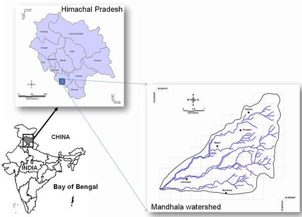
Abstract: Inventorying, mapping and monitoring landscape dynamics is essential for the sustainable management of natural resources including land and water. This work uses the temporal remote sensing data (1982, 1989, 2000 and 2007) for understanding landscape dynamics of Mandhala watershed in an ecologically fragile Himalayan region. Changes in land use and land cover are studied through established change detection techniques such as principal component analysis, correspondence analysis and NDVI based image differencing. Changes in forest land use are characterized by developing a forest fragmentation model involving various spatial metrics. The forest fragmentation and landscape metrics illustrate an increase in patch forests after 2000 and decline in the interior dense forest (90.4% to 33.4%) suggesting immediate policy interventions to restore the degraded landscape which had telling influence on local ecology, biodiversity and hydrology.

Keywords: landscape, land use change detection, forest fragmentation, watershed, multivariate analysis, Western Himalaya

1. Introduction

Land use and Land cover (LULC) information is a vital input for various developmental, environmental and resource planning applications at regional as well as global scale process models. LULC dynamics are analysed through changes in the state of an object or phenomenon by observing it at different times (Singh, 1989). Timely and accurate change detection of natural resources constitutes the foundation for greater understanding of the relationships and interactions between human and natural phenomena. It enables monitoring temporal dynamics of spatial aspects involving diverse ecosystems, forest changes, etc. Furthermore, remote sensing data pertaining to LULC provide spatio-temporal information of agricultural crops, wastelands, seasonal dynamics of wetlands/surface water bodies, forest, vegetation etc. which helps in analyzing reliably the landscape dynamics (Kandrika and Roy, 2008). 

Land use (LU) change can be obtained from multi satellite sensor data (spatio temporal data) using pre-classification or post-classification and pattern recognition algorithms (Duda et al., 2005). These classification algorithms can be either supervised, unsupervised, hybrid of soft classification techniques. In addition to the normal routine methods of estimating the LULC change in a landscape, landscape metrics or spatial metrics are being used in recent times particularly in landscape ecology (Gustafson, 1998). Spatial metrics are spatially consistent and provide detailed information about structures and patterns (Herold et al., 2005) and are being used to quantify shape and pattern of vegetation in natural landscape based on categorical, patch-based representation at a landscape, class and patch level (McGarigal and Marks, 1995). Computation of spatial metrics using multi-scale or temporal datasets, aids in assessing the changes in the degree of spatial heterogeneity. Thus, the information derived from several change detection techniques along with spatial metrics on temporal scales help in understanding the change phenomenon that benefits the planning and management towards a sustainable use of land resources. In this context, the present paper analyses the spatio-temporal landscape dynamics of Mandhala, a medium altitude, temperate watershed in Himachal Pradesh, India. Main objectives are to understand landscape dynamics through (i) LULC analysis using temporal remote sensing data (1972, 1989, 2000 and 2007) and (ii) computation of spatial metrics including forest fragmentation indices.

2. Tools and Techniques

This includes fusion of multi-resolution data (of different spectral and spatial resolutions), classification of data to derive land use parameters, fragmentation analysis to understand the process of fragmentation at the landscape level and computation of spatial metrics to capture landscape dynamics.

2.1. Image Fusion
Earth observation satellites provide data at different spatial, spectral and temporal resolutions. Satellites, such as IRS (LISS III) have a high spatial resolution panchromatic (PAN) band (5.8 m) and low resolution multispectral (MS) bands (G, R, NIR of 23.5 m) in order to support both spectral and best spatial resolution while minimising on-board data handling needs (Cakir and Khorram, 2008). For many applications, the fusion of these data from multiple sensors aids in delineating objects with comprehensive information due to the integration of spatial information present in the PAN image and spectral information present in the low resolution MS data. Here we have used the À Trous algorithm based wavelet transform (ATW) for image fusion (Nunez et al., 1999).

2.2. Image Classification
The extraction of LU information from remote sensing data is often difficult since it is closely associated with the human intervention for which the data need to be obtained from other sources (Kandrika and Roy, 2008). Keeping all the requirements and constraints in view, Gaussian Maximum Likelihood classifier (GMLC) is a parametric classifier used for classifying the satellite data.

2.3. Change detection
LU change detection is performed by change/no-change recognition followed by boundary delineation on images of two different time periods (Zhang and Zhang, 2007; Lu et al., 2004). Change/no-change recognition extracts changes from an unchanged background. The pixel patches marked as changed are then checked and the boundaries are delineated to extract the changed areas. A variety of change detection algorithms such as Principal Component Analysis (Zhang and Zhang, 2007), Correspondence Analysis (Cakir et al., 2006) and image differencing (Lyon et al., 1998) have been tested to recognise LU changes from bi-temporal images.

2.4. Forest fragmentation
Forest fragmentation is the process whereby a large, contiguous area of forest is both reduced in area and divided into two or more fragments (Meyer and Turner, 1994). The primary concern is direct loss of forest area, and all disturbed forests are subject to edge effects of one kind or another. Forest fragmentation metrics with the total extent of forest and its occurrence as adjacent pixels is computed through fixed-area windows surrounding each forest pixel. The result is stored at the location of the centre pixel. It is computed through Pf (the ratio of pixels that are forested to the total non-water pixels in the window) and Pff (the proportion of all adjacent (cardinal directions only) pixel pairs that include at least one forest pixel, for which both pixels are forested). Based on the knowledge of Pf and Pff, six fragmentation categories were mapped (Riitters et al., 2000): (i) interior, for which Pf = 1.0; (ii), patch, Pf < 0.4;  (iii) transitional, 0.4 < Pf < 0.6; (iv) edge, Pf > 0.6 and Pf – Pff > 0; (v) perforated, Pf > 0.6 and Pf – Pff < 0, and (vi) undetermined, Pf > 0.6 and Pf = Pff.

3. Study area

Mandhala watershed (figure 1) lies in Solan district, Himachal Pradesh, India (76°50'04'' to 76°53'47'' E and 30°53'40.7'' to 30°56'18.5'' N) and falls in lower Shiwalik range in the Himalayas at 400-1100 amsl spread over an area of 14.5 sq km, characterized by dry evergreen forests. Degradation of forest is evident from the dominant cover of invasive exotic species Lantana camera. Trees of Holoptelia integrifolia, Dalbergia sisoo, Morus nigra, etc. occur along the field bunds and other open lands.

Figure 1: Study area: Mandhala Watershed

The Western Himalayan climate is differentiated by the effect of altitude, topography and geographical trend causing reduced precipitation, extreme temperatures and increasing snowfall (Gaston et al., 1983). The forests in the watersheds are managed as reserve forest by the state forest department, cutting of trees is prohibited, still lopping and collection of fallen wood for household and industrial purposes were noticed during the field survey.

4. Methods

The methods adopted in the analysis included image fusion, LULC analyses, change detection using temporal data and temporal forest fragmentation analysis.

4.1. Data Preprocessing: Base layers like district boundary, drainage network, water bodies, etc. were mapped from the Survey of India (SOI) toposheets of scale 1:50000. Landsat bands, IRS LISS III MS bands were geocorrected with the known ground control points (GCP’s) and projected to geographic latitude-longitude with WGS-84 as the datum, followed by masking and cropping of the study region (region of interest – ROI). Resampling of the data using nearest neighbourhood technique were carried out for (i) bands 1- 4 of Landsat (1972) data to 79 m, (ii) bands 1-6 of Landsat TM (1989) to 30 m, (iii) bands 1-5 and 7 of Landsat ETM (2000) to 30 m and band 8 to 15 m, (iv) IRS LISS-III MS (2007) bands 1-3 to 23.5 m and IRS PAN band to 5.8 m. IRS PAN band of 5.8 m spatial resolution was merged with the LISS-III MS bands of 2007 using Multi-resolution analysis based on the wavelet transformation (Nunez et al., 1999). Landsat ETM+ PAN band (band 8) of 15 m spatial resolution was fused with bands 1, 2, 3, 4, 5 and 7 of the same satellite. Subsequently, all bands were resampled to 5.8 m for consistency and easier comparison of LU class statistics across the data sets.

4.2. LULC analysis: NDVI was computed to segregate regions under vegetation, soil and water. Signature separation corresponding to the LU classes was done using Transformed divergence (TD) matrix and Bhattacharrya (or Jeffries-Mastusuta) distance. Both the TD and Jeffries-Mastusuta measures are real values between 0 and 2, where ‘0’ indicates complete overlap between the signatures of two classes and ‘2’ indicates a complete separation between the two classes. Both measures are monotonically related to classification accuracies. The larger the separability values, the better the final classification results (Richards, 1986). Supervised classification using MLC with the training sets uniformly distributed representing / covering the study area was performed on the four temporal datasets. Accuracy assessment was done using error matrix by computing producer's accuracy, user's accuracy, overall accuracy and Kappa statistics (Campbell, 2002; Lillesand and Kiefer, 2002) by overlaying the test data not used in classification. Receiver operating characteristic (ROC) curves were plotted to assess the accuracy of the classified data (Fawcett, 2006). In the absence of historical data, the classified images of 1972, 1989 and 2000 were validated by visual interpretation using the tone, texture and other interpretation keys from the false colour composite images.

4.3. Spatial change analysis: Pixel to pixel change was mapped for each category from 1972 to 2007 using PCA - Principal Component Analysis (Zhang and Zhang, 2007), CA - Correspondence Analysis (Cakir et al., 2006) and NDVI image differencing (Lyon et al., 1998). The absolute and relative changes on the original bands of the two time periods were also computed. If there is a change between the two dates, the pixel had either negative or positive values. However, subtle change in brightness values between two dates also occur due to atmospheric conditions at different dates, sensor differences, etc., even after radiometric normalisation. Brightness values of no-change areas were distributed around the mean value of each difference image.

4.4. Forest fragmentation analysis: Pf and Pff in a kernel of 3 x 3 were computed (Riitters et al., 2000) to identify forest fragmentation categories. Based on these forest fragmentation indices (Hurd et al., 2002) Total forest proportion (TFP: ratio of area under forests to the total geographical extent excluding water bodies), weighted forest area (WFA) and Forest continuity (FC) were computed. TFP provides an extent of forest cover in a region ranging from 0 to 1. Weighted values for the weighted forest area (WFA) are derived from the median Pf value for each fragmentation class as given by equation 1 and FC is computed by equation 2.

                                  (1)

                                              (2)

Six patch level metrics – largest patch index, number of patches, patch density, total edge, edge density and landscape shape index were calculated using Fragstats (McGarigal et al., 2002).

5. Results and Discussion
Temporal NDVI analysis shows reduction of region under vegetation by 7.27% from 1972 to 2000 and a decrease of 4.72% from 1972 to 2007. Histograms were generated to ascertain the number of likely LU categories based on the number of distinguishable peaks. Six distinct classes: agriculture, settlement, forest, plantation/orchard, barren land and water were the dominant categories in the study area. Signatures were assessed using spectral graphs which showed that forest and plantation/orchard classes have high peaks in the NIR band and are therefore distinguishable from other classes. In band 3 of Landsat MSS settlement and dry river bed were not distinguishable, whereas in Landsat ETM+ for the same band, river bed was not easily distinguishable from barren land/stony/waste. In LISS III, settlement and barren land signatures were not separable in band 3. All other classes were well separable. Supervised classification (figure 2) with the percentage statistics are listed in table 1.

Table 1: Spatio-temporal LU estimates

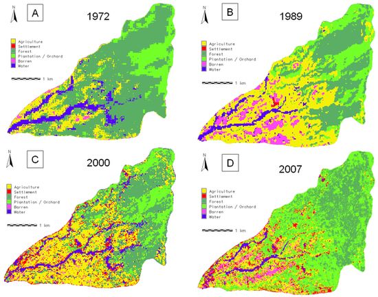
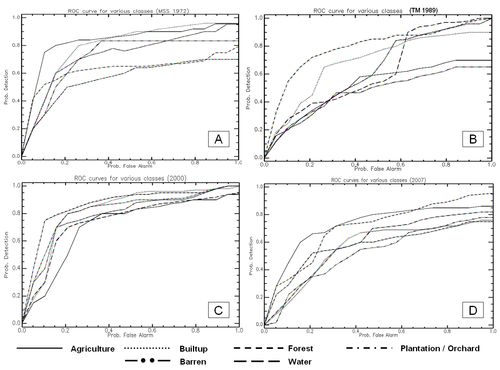
Figure 2: Classification using (A) Landsat MSS, 1972, (B) Landsat TM, 1989, (C) Landsat ETM, 2000 and (D) IRS LISS-III, 2007.

Accuracy assessment is listed in table 2. ROC curves for each class for the temporal dataset in figure 3 show the performance of the classifier as the decision threshold is varied for each class to obtain the best classified output. At any point on the curve is a possible operational point for the classifier and so was evaluated in the same manner as accuracy. There is a good agreement between results obtained from error matrix and ROC curves.

Figure 3: ROC curves for [A] Landsat MSS-1972; [B] Landsat TM – 1989; [C] Landsat ETM+ - 2000; [D] LISS-III - 2007.

Table 2: Accuracy assessment for classified images

Results obtained from MLC classification are comparable to the ground condition for the 2007 classified image. The successful application of MLC is dependent upon having delineated correctly the spectral classes in the image data of interest. This is necessary since each class is to be modeled by a normal probability distribution. If a class happens to be multimodal, and this is not resolved, then clearly the modelling cannot be very effective. MLC can obtain minimum classification error under the assumption that the spectral data of each class is normally distributed. The disadvantage of this technique is that it requires every training set to have at least one more pixel than the number of bands used in classification.

Forest patches have declined from 61 ha (in 1972) to 23 ha (in 2007) with the conversions of forest for agricultural activities, which has significantly increased by ~20% from 1972 to 2000. However, the percentage area pertaining to agriculture has decreased to 17% in 2007. One of the reasons is that agricultural area and fallow land were invaded by an exotic weed – Lantana camera which is an invasive species that thrives in warm, high rainfall areas where it forms dense thickets that exclude native species through shading and allelopathic effects, leading to complete dominance of the under storey and eventually overshooting the main canopy. The thickets impede access, alter availability of fodder for wild animals and reduce regeneration potential displacing natural scrub communities. Lantana encroaches agricultural land, reduces the carrying capacity of pastures. Its distribution has adversely affected not only many species of economic and ecological importance but ecosystem also. Plantation has increased considerably from ~15% (1972) to ~46% (2007). These include Babool, Acacia catechu and shrubs as a government measure to retain greenery in the area. Barren lands mainly constitute rocks, stones and open lands. Some of the barren land pixels show similar reflectance as that of dry river bed and the signatures often mix with settlements causing confusion during classification. Hence the proportion of barren land is less compared to earlier classified images (from 1989 to 2007).

Change detection involved differencing images of two time periods between PCs, CA components, NDVI and bands (rescaled from -1 to 1) that showed similar results. In both the images of the standardised PCA, PC1 had the highest information having all bands with unequal variances. CA puts less emphasis on bands that have low polarisation. The more the pixels are polarised for a band, the higher the importance given to that band in the calculation of the between-pixel distances (Greenacre, 1984). The first two components of CA explained approximately 99% of the total inertia in both temporal images (table 3). Total inertia is a measure of how much the individual pixel values are spread around the centroid. Inertia is independent of the absolute frequencies that constitute the original data, and will be identical if the data are multiplied by any constant value (Greenacre, 1984).

Table 3: Eigen structure of 1972 and 2007 data after PCA and CA transformation

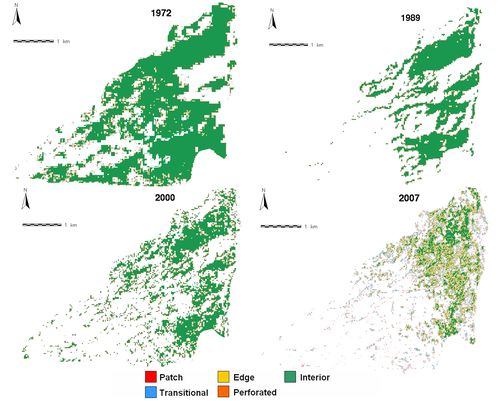
Detailed change detection tabulation was done between two classified images of 1972 and 2007 focusing primarily on the initial state classification changes – that is, for each initial state class, it identifies the classes into which those pixels changed in the final state image. The total class change for agriculture is 135.81 ha. There is a decrease of 537.03 ha in forest class and there has been an increase of 436.22 ha in plantation / orchard class. Forest fragmentation maps along with associated statistics based on the temporal forest maps (LU analysis) are presented in figure 4 and table 4.

Table 4: Forest fragmentation types details

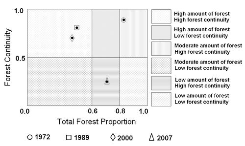
Figure 4: Forest fragmentation maps for 1972, 1989, 2000 and 2007.

Total forest proportion (TFP) and forest continuity (FC) is listed in table 5 and are depicted in figure 5. The forest fragmentation metrics analysis showed that largest forest patch is continuously decreasing consequently increasing the number of small patches and patch density. Due to increasing number of patches, more edges are getting developed with increasing edge density and the landscape shape is becoming more complex with time.

Figure 5: Six forest fragmentation conditions based on the values for TFP and FC.

Table 5: Total forest area and weighted forest area

The results of this study based on the temporal remote sensing data supplemented with the field data indicate that Mandhala watershed is degrading due to intense anthropogenic activities. When anthropogenic causes of fragmentation are considered, forest are more likely to be disturbed and fragmented where climate is hospitable, soil is productive and access is easy. Mandhala watershed is under the severe influence of forest fragmentation, calling for immediate protection measures from the concerned authorities.

5. Conclusions

Temporal remote sensing data showed reduction of vegetation by 7% from 1972 to 2000 and a decrease of 4.72% from 1972 to 2007. The reason for increase in vegetation from 2000 to 2007 is the spread of invasive species Lantana camera in and around the watershed. Change detection methods revealed a declining trend of forest patches (38%) during the last three decades due to increase in plantation and settlement area which was absent in 1972 and has significantly increased to ~7% (99 ha) in 2007. Forest fragmentation model showed that interior forest has declined by 57% (from 752 ha in 1972 to 106 ha in 2007). Patch forest which was absent till 2000, has increased up to 23 ha in 2007. Patches comes from many sources, ranging from our abilities to visualise and delineate what they represent, to their usage as conceptual units and patch dynamics models and to societal biases such as land ownership and anthropogenic activities. However, forest fragmentation which is degrading the ecosystem of the watershed requires immediate protection measures from the concerned authorities.

References

1. Cakir, H. I., and Khorram, S., Pixel Level Fusion of Panchromatic and Multispectral Images Based on Correspondence Analysis. Photogrammetric Engineering & Remote Sensing 2008, 74(2), 183-192.
2. Cakir, H. I., Khorram, S., Nelson, S.A.C., Correspondence analysis for detecting land cover change. Remote Sensing of Environment 2006, 102, 306–317.
3. Campbell, J. B., Introduction to Remote Sensing; Taylor and Francis: New York, 2002.
4. Duda, R.O., Hart, P.E., and Stork, D.G., Pattern classification, 2nd Ed., john Wiley & Sons, Inc: Canada, 2005.
5. Fawcett, T. An introduction to ROC analysis. Pattern Recognition Letters 2006, 27, 861-874.
6. Gaston, A. J., and Garson, P. J., and Hunter, M. L., The status and conservation of forest wildlife in Himachal Pradesh, Western Himalaya. Biological conservation 1983, 27, 291-314.
7. Greenacre, M., Theory and applications of correspondence analysis, Academic Press: London, 1984.
8. Gustafson, E. J., Quantifying landscape spatial pattern: What is the state of the art? Ecosystem 1998, 1, 143-156.
9. Herold, M., Couclelis, H., and Clarke, K.C., The role of spatial metrics in the analysis and modeling of urban land use change. Computers, Environment and Urban Systems 2005, 29, 369-399.
10. Hurd, J. D., Wilson, E. H., and Civco, D. L., Development of a Forest Fragmentation Index to Quantify the rate of forest change. In ASPRS-ACSM Annual Conference and FIG XXII Congress, April 22-26, 2002.
11. Kandrika, S., and Roy, P. S., Land use land cover classification of Orissa using multi-temporal IRS-P6 awifs data: A decision tree approach. International Journal of Applied Earth Observation and Geoinformatics 2008, 10, 186-193.
12. Lillesand, T. M., Kiefer. R. W., Remote Sensing and Image Interpretation, 4th Ed.; John Wiley and Sons: New York, 2002.
13. Lu, D., Mausel, P., Brondizio, E., and Moran, E. Change detection techniques. International Journal of Remote Sensing 2004, 25(12), 2365-2407.
14. Lyon, J. G., Yuan, D., and Lunetta, R. S., Elvidge, C.D.; A change detection experiment using vegetation indices.  Photogrammetric Engineering and Remote Sensing 1998, 64, 143-150.
15. McGarigal, K., Cushman, S.A., Neel, M.C., and Ene, E., FRAGSTATS: Spatial Pattern Analysis Program for Categorical Maps. Computer software program produced by the authors at the University of Massachusetts, Amherst, 2002. Available at: http://www.umass.edu/landeco/research/fragstats/fragstats.html
16. McGarigal, K., and Marks, B. J. FRAGSTATS: spatial pattern analysis program for quantifying landscape structure. USDA Forest Serv. Gen. Tech. Rep. PNW-351, 1995.
17. Meyer, W. B., and Turner, B. L., Changes in land use and land cover: a global perspective, Cambridge University Press: Cambridge, UK, 1994.
18. Nunez, J., Otazu, X., Fors, O., Prades, A., Pala, V., and Arbiol, R., Multiresolution-Based Image Fusion with Additive Wavelet Decomposition. IEEE Transactions of Geoscience and Remote Sensing 1999, 37(3), 1204-1221.
19. Richards, J. A., Remote Sensing Digital Image Analysis, Springer-Verlag: Berlin, 1986.
20. Riitters, K., Wickham, J., O' Neill, R., Jones, B., and Smith, E., Global-scale patterns of forest fragmentation. Conservation Ecology 2000, 4(2).
21. Singh, A., Digital change detection techniques using remotely sensed data. International Journal of Remote Sensing 1989, 10, 989-1003.
22. Zhang, J., Zhang, Y. Remote Sensing research issues of the National Land Use Change Program of China. Photogrammetry & Remote Sensing 2007, 62(6), 461-472.

BACK  «  TOP  »  NEXT