Abstract Land cover (LC) and land use (LU) dynamics induced by human and natural processes play a major role in global as well as regional patterns of landscapes influencing biodiversity, hydrology, ecology and climate. Changes in LC features resulting in forest fragmentations have posed direct threats to biodiversity, endangering the sustainability of ecological goods and services. Habitat fragmentation is of added concern as the residual spatial patterns mitigate or exacerbate edge effects. LU dynamics are obtained by classifying temporal remotely sensed satellite imagery of different spatial and spectral resolutions. This paper reviews five different image classification algorithms using spatio-temporal data of a temperate watershed in Himachal Pradesh, India. Gaussian Maximum Likelihood classifier was found to be apt for analysing spatial pattern at regional scale based on accuracy assessment through error matrix and ROC (receiver operating characteristic) curves. The LU information thus derived was then used to assess spatial changes from temporal data using principal component analysis and correspondence analysis based image differencing. The forest area dynamics was further studied by analysing the different types of fragmentation through forest fragmentation models. The computed forest fragmentation and landscape metrics show a decline of interior intact forests with a substantial increase in patch forest during 1972 - 2007. Key words: Land cover, algorithms, ROC curve, spatial change, correspondence analysis, forest fragmentation Introduction Numerous statistical classification algorithms exist, each one having a genesis behind its evolution. Depending on the nature of the data sources and methodology, multi-source, multi-sensor, multi-temporal, multi-frequency or multi-polarisation data are being used [2, 3, 4]. In most of the cases, the algorithms perform well with high degrees of accuracy, however, in an undulating terrain, where there is a large variation in spectral response due to high relief and shadow, the performance of a classifier deteriorates. Another major problem with these classifiers is their inability to classify data at different measurement scales and units due to invalid assumptions of statistical distributions. Temporal analysis of the spatial data provides an idea of the extent of changes happening in the landscape. LU details derived from temporal remote sensing (RS) data offer potential for assessing the changes in land uses, forest fragmentation and its impact on biodiversity, economics, greenhouse gas emission and hydrology. Spatial LU maps indicate only the location and type of forest, and further analyses are needed to quantify forest fragmentation. Hence, fragmentation of forests was assessed to understand the implication of temporal dynamics on forest habitats. Forest fragmentation is the process whereby a large, contiguous area of forest is both reduced in area and divided into two or more fragments. The decline in the size of the forest and the increasing isolation between the two remnant patches of the forest has been the major cause of declining biodiversity [5]. The primary concern is direct loss of forest area, and all disturbed forests are subject to “edge effects” of one kind or another. Forest fragmentation is of additional concern, insofar as the edge effect is mitigated by the residual spatial pattern [6]. In this context, objectives of this communication is to
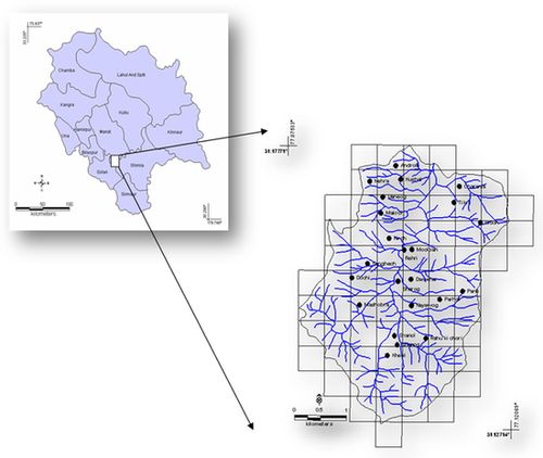
Material and Methods DATA Survey of India (SOI) toposheets of 1:50000 and 1:250000 scales were digitised to derive base layers. Ground control points (GCPs) for geo-rectification and training data for supervised classification of RS data were collected through field investigations using a handheld GPS. Google Earth data (http://earth.google.com) were used pre and post classification and also for validation. The RS data used for the study are Landsat MSS (79 m, 4 bands, acquired: November 15, 1972), Landsat TM (30 m, 6 bands, acquired: October 9, 1989), Landsat ETM+ (30 m, bands 1-5 and 7, band 8 - Panchromatic of 15m, acquired: October 15, 2000) and IRS LISS-III (23.5 m, 3 bands, acquired: May 9, 2007). Landsat data were downloaded (from http://glcf.umiacs.umd.edu/data/) and IRS data were procured from National Remote Sensing Centre, Hyderabad, India. Bands were geocorrected with the known GCP’s, and projected to geographic latitude-longitude with WGS-84 datum, followed by masking and cropping of the study area. Landsat data (of 1972) were resampled to 60 m, Landsat TM data of 1989 and IRS LISS III were resampled to 15 m using nearest neighbourhood technique. Study area: Moolbari watershed is situated in Shimla district, Himachal Pradesh, India as a part of Yamuna river basin and encompasses an area of 13.41 sq. km. from 31.07-31.17°N 77.05-77.15°E (figure 1). The altitude ranges from 1400 – 2000 m amsl. Figure 1: Moolbari watershed The vegetation in Moolbari is of mid-temperate comprising mixed deciduous (up to 1500 m) and sub-tropical pine forest (above 1500 m) in two different altitudinal ranges. There are reserve forests managed by state forest department, insofar cutting of trees is prohibited. However, lopping and collection of fallen wood for household purposes by the villagers are noted. METHODS The methods adopted in the analysis involve principal component analysis (PCA) based fusion, Land cover (LC), Land use (LU) analyses, change detection and forest fragmentation analysis. 1. Image Fusion: This was done using PCA fusion to increase the spatial resolution of multichannel image by introducing an image with a higher resolution. PC analysis was performed separately on the 6 bands of Landsat TM of 1989 (of spatial resolution 15 m) and 4 bands of Landsat MSS data of 1972 (of spatial resolution 60 m). PC1 of Landsat TM 1989 was stretched to have same mean and variance as that of PC1 of Landsat MSS using equation 1 [7].
where DNnew_image is the image that has same mean and variance as that of principal component (PC) 1 of Landsat MSS, μref and σref refers to the mean and standard deviation of PC1 of Landsat MSS. DNold, μold and σold represent the digital number, mean and standard deviation of PC1 of Landsat TM (1989). PC1 of Landsat MSS was replaced with PC1 of higher resolution Landsat TM of 1989 as it contains the information which is common to all bands while the spectral information is unique for each band. PC1 accounts for maximum variance which can maximise the effect of the high resolution data in the fused image. Finally, high-resolution multispectral images were determined by performing the inverse PCA transformation. Similarly, Panchromatic band at 15 m resolution was fused with the 6 bands (at 30 m) of Landsat ETM+ (2000). With this, the RS data corresponding to 4 time periods were at a uniform spatial resolution of 15 m for easy analysis, consistency and multi-date pixel to pixel comparison. These data were used subsequently for LU classification and spatial change analysis. 2. Land cover (LC): NDVI was computed to segregate regions under vegetation, soil and water using NIR and Red bands of temporal data. 3. LU classification: The classification techniques evaluated on temporal data (with diverse spatial and spectral resolutions) are: Gaussian Maximum Likelihood Classifier (GMLC), Minimum distance to means, Mahalanobis distance, Parallelepiped and Binary Encoding (BE).
Accuracy assessment of these techniques was done using error matrix and receiver operating characteristic (ROC) curves to choose the best classifier. 4. LU change detection: This is performed by change/no-change recognition followed by boundary delineation on images of multi time periods [15]. Changes across a period of 35 years were analysed through PCA, correspondence analysis (CA) and Normalised Difference Vegetation Indices (NDVI) differencing based change detection.
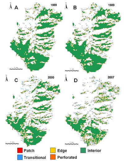
5. Forest Fragmentation: Forest fragmentation analysis was done to quantify the type of forest in the study area - patch, transitional, edge, perforated, and interior based on the classified images. Additionally, landscape metrics were computed to understand the fragmentation process at a patch and class level. These metrics along with the state of the forest fragmentation index was used to quantify and investigate the fragmentation process. Forest fragmentation statistics and the total extent of forest and its occurrence as adjacent pixels is computed through fixed-area windows surrounding each forest pixel, which is used to classify the window by the type of fragmentation. The result is stored at the location of the centre pixel. Thus, a pixel value in the derived map refers to between-pixel fragmentation around the corresponding forest location [21]. Forest fragmentation category at pixel level is computed through Pf (the ratio of pixels that are forested to the total non-water pixels in the window) and Pff (the proportion of all adjacent (cardinal directions only) pixel pairs that include at least one forest pixel, for which both pixels are forested. Pff estimates the conditional probability that, given a pixel of forest, its neighbour is also forest. Based on the knowledge of Pf and Pff [21], six fragmentation categories: (1) interior, when Pf = 1.0; (2), patch, when Pf < 0.4; (3) transitional, when 0.4 < Pf < 0.6; (4) edge, when Pf > 0.6 and Pf – Pff > 0; (5) perforated, when Pf > 0.6 and Pf – Pff < 0, and (6) undetermined, when Pf > 0.6 and Pf = Pff are mapped. Based on these forest fragmentation indices, Total forest proportion (TFP: ratio of area under forests to the total geographical extent excluding water bodies), weighted forest area (WFA) and Forest continuity (FC) are computed. TFP provides a basic assessment of forest cover in a region ranging from 0 to 1. Weighted values for the weighted forest area (WFA) are derived from the median Pf value for each fragmentation class as given by equation 2 below:
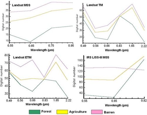
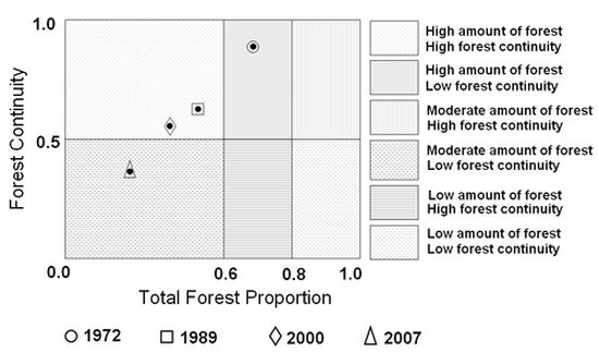
TFP designations are as per Vogelmann (1995) [22] and Wickham et al.(1999) [23]; Forest fragmentation become more severe as forest cover decreases from 100 percent towards 80 percent. Between 60 and 80 percent forest cover, the opportunity for re-introduction of forest to connect forest patches is the greatest, and below 60 percent, forest patches become small and more fragmented. The FC regions were evenly split and designated as high forest continuity (above 0.5) or low forest continuity (below 0.5). FC value examines only the forested areas within the analysis region. The rationale is that given two regions of equal forest cover, the one with more interior forest would have a higher weighted area, and thus be less fragmented. To separate further regions based on the level of fragmentation, the weight area ratio is multiplied by the ratio of the largest interior forest patch to total forest area for the region. FC ranges from 0 to 1. Results and discussion NDVI was computed with the temporal data of 1972, 1989, 2000 and 2007 for land cover analysis to delineate area under green (agriculture, forest and plantations /orchards) and non-green (builtup land, waste / barren rock and stones). This shows the reduction of region under vegetation by 5.59% during three decades. Further analyses of four datasets were done using Iterative Self-Organising Data (ISO data) [24, 25] clustering to understand the number of probable classes. It indicated that the mapping of the classes could be done accurately, giving an overall good representation of what was observed in the field. Initially 25 clusters were made, and clusters were merged one by one to produce a map with three distinct classes: forest, agriculture and barren land that were the dominant categories in the study area. Signature separability of the LU classes was done using Transformed divergence (TD) matrix and Bhattacharrya (or Jeffries-Mastusuta) distance and spectral graphs (figure 2). Both the TD and Jeffries-Mastusuta measures are real values between 0 and 2, where ‘0’ indicates complete overlap between the signatures of two classes and ‘2’ indicates a complete separation between the two classes. Both measures are monotonically related to classification accuracies. The larger the separability values, the better the final classification results. The possible ranges of separability values are 0.0 to 1.0 (very poor); 1.0 to 1.9 (poor); 1.9 to 2.0 (good). Very poor separability (0.0 to 1.0) indicates that the two signatures are statistically very close to each other [26]. Figure 2 shows that all the classes are well separable except barren and agriculture in band 4 of Landsat TM/ETM and IRS LISS-III data. Supervised classification was performed for land use analysis based on the training data uniformly distributed representing / covering the study area using the five algorithms. GMLC output is shown in figure 3. The error matrix [27] is given in table 1 and ROC curves [28] were plotted for each class (figure 4) to assess the accuracy of the classified data. Table 1: Overall accuracy and kappa statistics for each classifier (OA - Overall Accuracy)
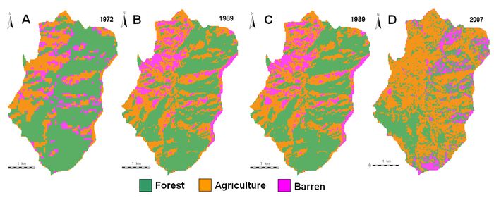
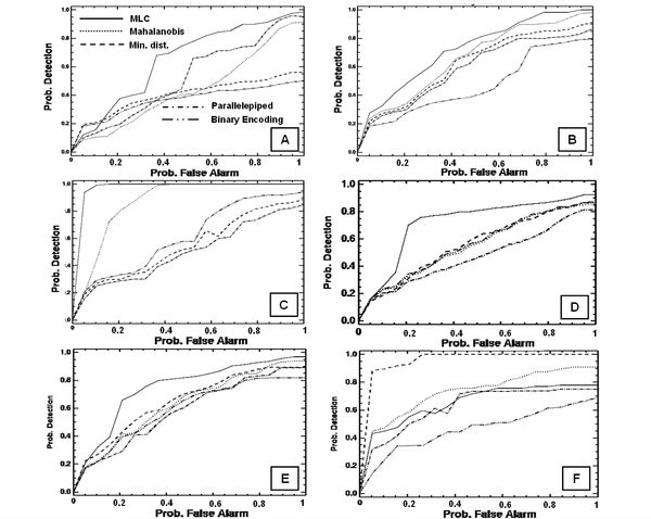
Figure 2: Spectral signature separability for various sensor data Figure 3: GMLC based LU classification using (A) Landsat MSS, 1972, (B) Landsat TM, 1989, (C) Landsat ETM, 2000 and (D) IRS LISS-III, 2007 ROC curve helped in visualising the performance of a classification algorithm as the decision threshold could be varied algorithm-wise for each class. The best possible classification would yield a point in the upper left corner or coordinate (0,1) of the ROC space, representing 100% sensitivity (all true positives are found) and 100% specificity (no false positives are found). The (0,1) point is also called a perfect classification. A completely random guess would give a point along a diagonal line (line of no-discrimination) from the left bottom to the top right corners. The diagonal line divides the ROC space in areas of good or bad classification. Points above the diagonal line indicate good classification results, while points below the line indicate wrong results [29]. Figure 4: ROC curves for [A] Forest (1972); [B] Agriculture (1972); [C] Barren (1972); [D] Forest (2007); [E] Agriculture (2007); [F] Barren (2007) for the five different classifiers There is a good agreement between results obtained from error matrix and ROC curves to the ranking of the performance of the classification algorithms. They indicate that GMLC is the best performing algorithm for different sensor datasets (table 2). This conventional per-pixel, spectral-based classifier constitutes a historically dominant approach to RS-based automated LU and LC derivation [30, 31]. In fact, this aids as “benchmark” for evaluating the performance of novel classification algorithms [32]. Table 2: Ranking of algorithms based on Overall accuracy
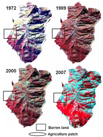
Results of all these algorithms are valid only for the particular architecture or parameter settings tested although there may be other architectures that offer better performance. Selection of parameters is done based on the training data, evaluation, and test set methodology. Finally, for one particular application, the best way to select a classifier and its operational point is to use the Neyman-Pearson method of selecting the required sensitivity and then maximising the specificity with this constraint (or vice versa). The spectral signature curve for IRS LISS-III shows confusion between barren and agriculture. A similar result was obtained in the Jeffries-Matusita matrix with the separability values of 1.4 (poor separability). This was also observed while performing the clustering on LISS-III data. The analysis showed GMLC to be better among the five algorithms. However, the successful application of GMLC is dependent upon having delineated correctly the spectral classes in the image data of interest. This is necessary because each class is to be modelled by a normal probability distribution. GMLC can obtain minimum classification error under the assumption that the spectral data of each class is normally distributed. The disadvantage is that it require its’ every training set to include at least one more pixel than the number of bands. If a class happens to be multimodal, and this is not resolved, then clearly the modelling cannot be very effective. Mahalanobis distance is similar to any other statistical classifier and uses Mahalanobis distance as a metric. It takes into account errors associated with prediction measurement such as noise, by using the feature covariance matrix to scale features according to their variances. This classifier performed well on 1972 and 2000 images. Minimum distance to means is mathematically simple and computationally efficient. However, it has more error of omission and commission. It is insensitive to different degrees of variance in spectral response data. Therefore it should not be used where spectral classes are close to one another in the measurement space and have high variance. Although Parallelepiped algorithm did not perform very well, it is known for its good computational speed. When pixels are within overlapped region of parallelogram, then it may perform unsatisfactorily as pixels will end up unclassified and lead to error of omission. BE did not perform very well for any dataset. However, this technique has been reported useful for high spectral resolution data where high-speed spectral signature matching is required. In order to effectively use this technique for spectral clustering, one must account for spectra which are relatively flat and devoid of absorption features. Spatial change in LU pattern from 1972 to 2007 is shown in table 3. There is a decline of forest patches (48%) during the last three decades due to increasing agricultural practices. Agricultural area has significantly increased from 264 hectares (1972) to 779 hectares (2007). Barren area has increased by 23% (during 1972 to 2000). Barren land mainly constitutes the rocks, stones, and built ups. However, the proportion of barren land in 2007 is less compared to earlier classified images as some pixels corresponding to barren areas with grass cover showed similar spectral aspects as agriculture, which can be ascertained from figure 5. Figure 5: FCC of Landsat MSS (1972), Landsat TM (1989), Landsat ETM (2000) and LISS-III (2007). FCC of 2007 shows similar reflectance of barren/stone and agricultural patch leading to confusion between these two classes Difference of temporal PCs, CA-PC’s, NDVI images and bands (rescaled from -1 to 1) showed similar results. To see the change in forest and agriculture, the NIR band of 1972 (T1) and 2007 (T2) were used which have the advantage of highlighting vegetation pixels because of the maximum reflectance by the green plants. The two NIR bands were first normalised by subtracting the image minimum and dividing by the image data range. Normalised temporal maps were then subtracted (T2 – T1) to see the absolute change in pixel values and were then converted to relative difference map with values ranging from -1 to +1 with 0 representing no change, -1 representing negative change and positive values representing increase in the value of the digital number of pixels from 1972 to 2007. Table 3: LU change from 1972, 1989, 2000 and 2007
In both the images of the non-standardized PCA, PC1 had the highest information having all bands with unequal variances. CA puts less emphasis on bands that have low polarisation. Higher is the importance given to that band in the calculation of the between-pixel distances if more number of pixels are polarised in a band. First two components of CA explained approximately 99% of the total inertia in both images (table 4). Total inertia is a measure of how much the individual pixel values are spread around the centroid. Table 4: Eigen structure of 1972 and 2007 data after PCA and CA transformation
Detailed change detection tabulation was done between two classified images of 1972 and 2007. The analysis focuses primarily on the initial state classification changes – that is, for each initial state class (in 1972), it identifies the classes into which those pixels changed in the final state image (in 2007). Changes are reported as pixel counts, area and percentages in table 5 that list the initial state classes in the columns and the final state classes in the rows for the paired initial and final state classes. The rows contain all of the final state classes (2007) which are required for complete accounting of the distribution of pixels that changed classes. Table 5: LU change detection statistics (1972 to 2007)
For each initial state class (i.e., each column), the table indicates how these pixels were classified in the final state image. In table 5, 18209 pixels (410.55 ha) initially classified as forest (in 1972) changed into agriculture class in the final state image (2007). 23025 pixels were classified as forest in the initial state image (in 1972). The Class Total Row indicates the total number of pixels in each initial state class, (42370 in the Forest column = 23025+18209+1136. similarly there are 10350 pixels in agriculture and 6759 pixels in barren class) in 1972. The Class Total Column indicates the total number of pixels in each final state class (29361 pixels were classified as agriculture in the final state image). The Row Total Column is simply a class-by-class summation of all the final state pixels that fell into the selected initial state classes. Sometimes this may not be the same as the Class Total Column (i.e. final state class total) because it is not required that all initial state classes be included in the analysis. For example, if there was a fourth class “water” in 1972 and were absent in 2007 classified image or not considered while classification then the Row Total Column would not be equal to Class Total Column because total number of pixels in any final state class will not be equal to summation of all the final state pixels in that class. The difference in the Row Total Column and Class Total Column are due to those pixels. However, in the present case, Row total Column indicates that there is no unclassified pixel as same numbers of pixels are also reported in the Class Total Column. The Class Changes Row indicates the total number of initial state pixel that changed classes. In table 5, the total class change for forest is 19345 pixels. In other words, 19345 pixels that were initially classified as forest changed into final state classes other then forest. To confirm that this is correct, the number of initial forest classified pixels 23025 are subtracted from the forest class total 42370, which is 19345. The Image Difference Row is the difference in the total number of equivalently classed pixels in the two images, computed by subtracting the initial state class totals from the final state class totals (i.e. Class Total Column - Class Total Row). An image difference that is positive indicates that the class size increased. The table shows that there is a decrease of 15604 pixels (352.27 ha) in forest class and there has been an increase of 19001 pixels (428.57 Ha) in agriculture class. Temporal analysis revealed large scale LC changes in the region. To understand the level of changes, fragmentation analysis was done, which would help in assessing the state of fragmentation and its implications. In this regard, Pf and Pff in a fixed-area window of 3 x 3 were computed [21] to identify forest fragmentation categories given in figure 6 and table 6. Table 6: Forest fragmentation types details
Figure 6: Forest fragmentation map (A) 1972, (B) 1989 (C) 2000 (D) 2007 The case of Pf = 1 (interior) represents a completely forested window for which Pff is also 1. When Pff is larger than Pf, the implication is that forest is clumped; the probability that an immediate neighbour is also forest is greater than the average probability of forest within the window. Conversely, when Pff is smaller than Pf, the implication is that whatever is nonforest is clumped. The difference (Pf-Pff) characterises a gradient from forest clumping (edge) to nonforest clumping (perforated). When Pff = Pf, the model cannot distinguish forest or nonforest clumping. To understand the fragmentation process, 10 spatial metrics – Number of patches (NP), Patch density (PD), Total edge (TE), Edge Density (ED), Largest shape index (LSI), Shannon diversity index (SHDI) were calculated at landscape level using Fragstats [33]. Quantitative assessment of the pattern of forest fragmentation and its trends showed that interior forest has declined by 68.81%. Patch forest which was absent in 1972 image has increased up to 12 ha in 2007 and interior forest has decreased from 789 ha in 1972 to 246 ha in 2007. The values of TFP and FC for the temporal data were plotted that specifies six conditions of forest fragmentation in figure 7. The amount of forest and continuity were high in 1972 and declined in 2007. Figure 7: Six forest fragmentation conditions based on the values for Total Forest Proportion and Forest calculated for a region Forest in Moolbari watershed was more contiguous earlier (in 1972), with less number of patches than that of 2007. There was a single contiguous patch of forest, which is now more fragmented with interspersion of agriculture land and reduced area (925 ha in 1972 to 474 ha) in 2007. Individually, the largest patch in 1972 was 907 ha, while in 2007, the largest patch is 273 ha. Number of patches and patch density, which are the direct measure of fragmentation effect also increased over years. Table 7 details the fragmentation metrics calculated at landscape level. Table 7: Forest fragmentation indices for 1972 to 2007
From this analysis, it is clear that Moolbari watershed in the ecologically fragile Himalaya is under the severe influence of forest fragmentation, necessitating immediate interventions involving integrated watershed management strategies. The results highlight higher anthropogenic fragmentation in the watershed closer to villages than remote areas. Conclusion LU classification algorithms were reviewed to assess the best classifier in an undulating terrain. Error matrix along with ROC curves provided a richer measure of classification performance showing that GMLC is superior with overall accuracy of 89% (1972 and 1989), 81% (2000) and 88% (2007). The study showed reduction of region under vegetation by 5.59% during 35 years. Change detection methods revealed a declining trend of forest patches (48%) during the last three decades due to increasing agricultural practices which have significantly increased from 264 ha (1972) to 779 ha (2007). Barren area has increased by 23% (during 1972 to 2000). Forest fragmentation model showed that interior forest has declined by 68.81% (from 789 ha in 1972 to 246 ha in 2007). Patch forest which was absent in 1972 image has increased up to 12 ha in 2007. Forested area is negatively correlated to all the indices, hinting that decreased forest area has more fragmented patches. Patches come from many sources, ranging from our abilities to visualise and delineate what they represent, to their usage as conceptual units and patch dynamics models and to societal biases such as land ownership and anthropogenic activities. The analysis places patches into perspective as one identifiable element along a continuum of forest fragmentation, and suggest that more attention should be given for the conservation of interior forests and restoration of patch forests for the sustainability of watershed, livelihood and food security. Acknowledgement We are grateful to the NRDMS division, DST, Ministry of Science and Technology, Government of India for the financial assistance and to National Remote Sensing Centre (NRSC), Hyderabad for providing the remote sensing data. Landsat data was downloaded from http://glcf.umiacs.umd.edu/data/). We thank Dr.Rana and his team at Shimla for the support during the field data collection. References
|
|||||||||||||||||||||||||||||||||||||||||||||||||||||||||||||||||||||||||||||||||||||||||||||||||||||||||||||||||||||||||||||||||||||||||||||||||||||||||||||||||||||||||||||||||||||||||||||||||||||||||||||||||||||||||||||||||||||||||||||||||||||||||||||||||||||||||||||||||||||||||||||||||||||||||||||||||||||||||||||||||||||||||||||||||||||||||||||||||||||||||||||||||||||||||||||||||||||||||||||||||||||||||||||||||||||||||||||||||||||||||||||||||||||||||||||||||||||||||||||||||||||||||||||||||||||||||||||||||||
 (1)
(1) from x to each of the mean vectors, and assign x to the closest category.
  so that
  and eigenvalues would be smaller than or equal to 1. Multispectral data are then transformed into the component space using the matrix of eigenvectors. Image differencing is applied to CA components to perform change detection.
  (2)
(2)  (3)
(3)