Land cover Assessment-Uttara Kannada District

T. V. Ramachandra, Senior Member, IEEE, Uttam Kumar, Student Member, IEEE
P. G. Diwakar and N. V. Joshi

Abstract — Landslide is induced by a wide range of ground movements, such as rock falls, deep failure of slopes, shallow debris flows, etc. These ground movements are caused when the stability of a slope changes from a stable to an unstable condition. A change in the stability of a slope can be caused by a number of factors acting together such as loss or absence of vegetation (changes in land cover), soil structure, etc. Loss of vegetation happens when the forest patch is fragmented that can be either anthropogenic or natural. Hence land cover mapping with forest fragmentation can provide an opportunity for visualising the areas that require immediate attention from slope stability aspects. In this paper, À Trous algorithm based wavelet transform is used to merge IRS 1D LISS-III MSS (23.5 m) and PAN (5.8 m) images. The fused images are classified using K-nearest neighbour for land cover categories . A fragmentation model is developed to analyse the extent of forest fragmentation in Uttara Kannada district, Karnataka, India. This helped in visualising the effect of land use changes in five west flowing river basins in the district. Field investigation of land slide region confirm that land cover plays a very vital role in landslides. Change in land cover in the catchment area of these rivers has triggered landslide.

Index Terms — Landslide, à trous, multiresolution

INTRODUCTION

A Landslide is a geological phenomenon involving small to medium to large ground movements caused due to change in stability of a slope to an unstable condition. Change in the stability of a slope can be induced by a number of factors, acting together or alone such as rock falls, deep failure of slopes, shallow debris flows, ground water pressure, loss or absence of vegetative cover, erosion, soil nutrients, soil structure, etc. Although the action of gravity is the primary driving force for a landslide to occur, there are other contributing factors affecting the original slope stability. The pre-conditional factors build up specific sub-surface conditions that make the area/slope prone to failure, whereas the actual landslide often requires a trigger before being released. A change in land cover due to the loss of vegetation is a primary factor that builds up specific sub-surface conditions for landslide to occur. The losses in vegetation cover results in fragmenting large, continuous area of forest into two or more fragments. Forest fragmentation apart from affecting the biodiversity and ecology of the region has a significant influence in the movement of soil (silt) and debris in an undulating terrains with high intensity rainfall. Forest fragmentation analysis spatially aids in visualizing the regions that require immediate attention to minimize landslides. Spatial fragmentation map depicts the type and extent of fragmentation. These  are derived from land use (LU) data which are obtained from multi-source, multi-sensor, multi-temporal, multi-frequency or multi-polarization remote sensing (RS) data. The objectives of this paper are

• Pixel based image fusion of LISS (Linear Imaging Self Scanner)-III MSS (Multispectral) images of 23.5 m spatial resolution with PAN (Panchromatic) image of 5.8 m spatial resolution using À Trous algorithm based wavelet transform (ATW).
• Classification of fused image using K-nearest neighbour to obtain LU map.
• Forest fragmentation analysis to characterise the type and extent of fragmentation or loss of vegetation cover.

Methods

Pixel based image fusion : Earth observation satellites provide data at different spatial, spectral and temporal resolutions. Satellites, such as IRS bundle a 4:1 ratio of a high resolution PAN band and low resolution MSS bands in order to support both colour and best spatial resolution while minimizing on-board data handling needs [1]. For many applications, the fusion of spatial and spectral data from multiple sensors aids in delineating objects with comprehensive information due to the integration of spatial information present in the PAN image and spectral information present in the low resolution MSS data. Pixel based image fusion refers to the merging of measured physical parameters or fusion at the lowest processing level of co-registered or geocoded data. Many fusion techniques are developed to integrate both PAN and MSS data considering, application of the user. In this communication we use the À Trous algorithm based wavelet transform (ATW).

Multiresolution analysis based on the wavelet theory (WT) is based on the decomposition of the image into multiple channels depending on their local frequency content. While the Fourier transform gives an idea of the frequency content in image, the wavelet representation is an intermediate representation and provides a good localisation in both frequency and space domain [2]. The WT of a distribution f(t) is expressed as

(1)

where a and b are scaling and transitional parameters, respectively. Each base function  is a scaled and translated version of a function ψ called Mother Wavelet. These base functions are . Most of the WT algorithms produce results that are not shift invariant. An algorithm proposed by Starck and Murtagh [3] uses a WT known as à trous to decompose the image into wavelet planes that overcomes this problem. Given an image p we construct the sequence of approximations: . by performing successive convolutions with a filter obtained from an auxiliary function named scaling function which has a B3 cubic spline profile. The use of a B3 cubic spline leads to a convolution with a mask of 5 x 5:

(2)

The wavelet planes are computed as the differences between two consecutive approximations pl-1 and pl. Letting wl = pl-1 - pl (l = 1, …, n), in which p0 = p, the reconstruction formula can be written as

(3)

The image pl (l = 0, …, n) are versions of original image p, wl (l = 1, …, n) are the multiresolution wavelet planes, and pr is a residual image. The wavelet merger method is based on the fact that, in the wavelet decomposition, the images pl (l = 0, …, n) are the successive versions of the original image. Thus the first wavelet planes of the high resolution PAN image have spatial information that is not present in the MSS image. In this paper, we follow the Additive method [2] where the high resolution PAN image is decomposed to n wavelet planes. For 1:4 fusion (as in IRS 1D) n is set to 2.

(4)

The wavelet planes of the PAN decomposition are added to the low resolution MSS images individually to get high resolution MSS images.

K-nearest neighbour classification : Two of the main challenges in RS data interpretation with using parametric techniques are high dimensional class data modeling and the associated parameter estimates. While the Gaussian normal distribution model has been adopted widely, the need to estimate a large number of covariance terms leads to a high demand on the number of training samples required for each class of interest. In addition, multimode class data cannot be handled properly with a unimodal Gaussian description. Nonparametric methods, such as K-nearest neighbour (KNN) have the advantage of not needing class density function estimation thereby obviating the training set size problem and the need to resolve multimodality [4]. The KNN algorithm [5] assumes that pixels close to each other in feature space are likely to belong to the same class. It bypasses density function estimation and goes directly to a decision rule. Several decision rules have been developed, including a direct majority vote from the nearest k neighbours in the feature space among the training samples, a distance-weighted result and a Bayesian version [6].

Let x be an unknown pixel vector and suppose there are ki neighbours labelled as class ωi out of k nearest neighbours.
 (M is the number of class defined). The basic KNN rule is
where
                                               (5)

If the training data of each class is not in proportion to its respective population, p(ωi), in the image, a Bayesian Nearest-Neighbour rule is suggested based on Bayes’ theorem

(6)

The basic rule does not take the distance of each neighbour to the current pixel vector into account and may lead to tied results every now and then. Weighted-distance rule is used to improve upon this as

(7)

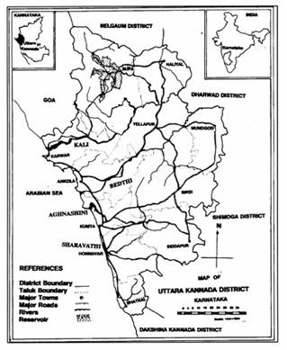
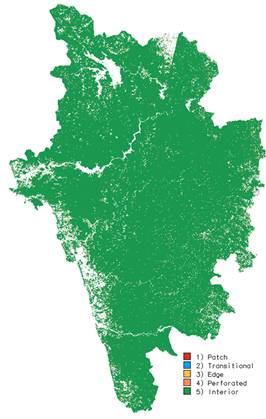
where dij is Euclidean distance. Assuming there are S training samples, one needs to find the k nearest neighbours from S training samples for every pixel in a large image. This means S spectral distances must be evaluated for each pixel. The above algorithm is summarised as follows:

The variable unknown denotes the number of pixels whose class is unknown and the variable wrong denotes the number of pixels which have been wrongly classified.
set No: of pixels = 0.
set unknown = 0.
set wrong = 0.
For all the pixels in the test image
do
{
1. Get the feature vector of the pixel and increment no. of pixels by 1.

2. Among all the feature vectors in the training set, find the sample feature vector which is nearest (nearest neighbor) to the feature vector of the pixel.

3. If the no. of nearest neighbors is more than 1, then

Check whether the corresponding class labels of all the nearest sample feature vectors are the same.

If the corresponding class labels are not the same, then increment unknown by 1 and go to Step 1 to process the next pixel else go to Step 4.

4. Class label of the image pixel=class label of the nearest sample vector. Go to Step 1 to process the next pixel.
}

Forest fragmentation : Forest fragmentation is the process whereby a large, continuous area of forest is both reduced in area and divided into two or more fragments. The decline in the size of the forest and the increasing isolation between the two remnant patches of the forest has been the major cause of declining biodiversity [7, 8, 9, 10 and 11]. The primary concern is direct loss of forest area, and all disturbed forests are subject to “edge effects” of one kind or another. Forest fragmentation is of additional concern, insofar as the edge effect is mitigated by the residual spatial pattern [12, 13 and 14].

LU map indicate only the location and type of forest, and further analysis is needed to quantify the forest fragmentation. Total extent of forest and its occurrence as adjacent pixels, fixed-area windows surrounding each forest pixel is used for calculating type of fragmentation. The result is stored at the location of the centre pixel. Thus, a pixel value in the derived map refers to between-pixel fragmentation around the corresponding forest location. As an example [15] if Pf is the proportion of pixels in the window that are forested and Pff is the proportion of all adjacent (cardinal directions only) pixel pairs that include at least one forest pixel, for which both pixels are forested. Pff estimates the conditional probability that, given a pixel of forest, its neighbour is also forest. The six fragmentation model that identifies six fragmentation categories are: (1) interior, for which Pf = 1.0; (2), patch, Pf < 0.4; (3) transtitional, 0.4 < Pf < 0.6; (4) edge, Pf > 0.6 and Pf-Pff > 0; (5) perforated, Pf > 0.6 and Pf-Pff < 0, and (6) undetermined, Pf > 0.6 and Pf = Pff. When Pff is larger than Pf, the implication is that forest is clumped; the probability that an immediate neighbour is also forest is greater than the average probability of forest within the window. Conversely, when Pff is smaller than Pf, the implication is that whatever is nonforest is clumped. The difference (Pf-Pff) characterises a gradient from forest clumping (edge) to nonforest clumping (perforated). When Pff = Pf, the model cannot distinguish forest or nonforest clumping. The case of Pf = 1 (interior) represents a completely forested window for which Pff must be 1.

Study area and Data

The Uttara Kannada district lies 74°9' to 75°10' east longitude and 13°55' to 15°31' north latitude, extending over an area of 10,291 km² in the mid-western part of Karnataka state (Fig. 1). It accounts for 5.37 % of the total area of the state with a population above 1.2 million [16]. This region has gentle undulating hills, rising steeply from a narrow coastal strip bordering the Arabian sea to a plateau at an altitude of 500 m with occasional hills rising above 600–860 m. This district, with 11 taluks, can be broadly categorised into three distinct regions –– coastal lands (Karwar, Ankola, Kumta, Honnavar and Bhatkal taluks), mostly forested Sahyadrian interior (Supa, Yellapur, Sirsi and Siddapur taluks) and the eastern margin where the table land begins (Haliyal, Yellapur and Mundgod taluks). Climatic conditions range from arid to humid due to physiographic conditions ranging from plains, mountains to coast.

Fig. 1. Uttara Kannada district, Karnataka, India

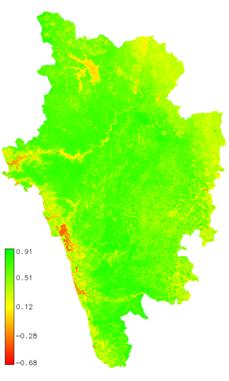
Survey of India (SOI) toposheets of 1:50000 and 1:250000 scales were used to generate base layers – district and taluk boundaries, water bodies, drainage network, etc. Field data were collected with a handheld GPS. RS data used in the study were LISS-III MSS (in Blue, Green and Red bands) and PAN band, procured from NRSA, Hyderabad, India. Google Earth data (http://earth.google.com) served in pre and post classification process and validation of the results.

Results and Discussion

RS data were geometrically corrected on a pixel by pixel basis. The low resolution MSS images (7562 x 4790) were upsampled to the size of high resolution PAN image (30284 x 19160). MSS and PAN data were fused using ATW method and the decomposition level (n) was set to 2. Land cover (LC) mapping (Fig. 2) was done using normalised difference vegetation index (NDVI) given as

(8)

NDVI values range from -1 to +1; increasing values from 0 indicate presence of vegetation and negative values indicate absence of greenery. LC analysis showed 94 % green (agriculture, forest and plantation) and remaining 6 % other categories (builtup, sand, fallow, water).

Fig. 2. LC of Uttara Kannada district.

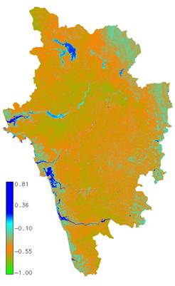
Mapping of water bodies (Fig. 3) was done using normalised difference water index (NDWI) [17] given as

(9)

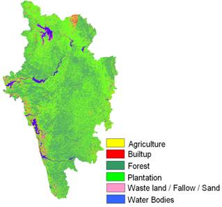
NDWI values above 0 indicate presence of water bodies and values below 0 indicate other classes. The major rivers in Uttara Kannada are showed in blue in Fig. 3 that constitute approximately 2.5 % (25000 ha) of the entire district.

The class spectral characteristics for six LU categories (agriculture, builtup, forest, plantation, waste land / fallow / sand, and water bodies) using LISS-III MSS bands 2, 3 and 4 were obtained from the training pixels spectra to assess their inter-class separability and the images were classified using KNN with training data uniformly distributed over the study area collected with pre calibrated GPS (Fig. 4). This was validated with the representative field data (training sets collected covering the entire city and validation covering ~ 10% of the study area) and also using Google Earth image.

Fig. 3. Water Index of Uttara Kannada district.

Fig. 4. LU in  Uttara Kannada district.

LU statistics, producer’s accuracy, user’s accuracy and overall accuracy computed are listed in table 1. Using the results from classification, forest fragmentation model was used to obtain fragmentation indices as shown in Fig. 5 and the statistics are presented in table 2. Forest and plantation were considered as a single class - forest and all other classes were considered as non-forest as the extent of land cover is a decisive factor in landslides. It is seen that majority of the area (97 %) is interior forest.

Fig. 5. Fragmentation of forests in Uttara Kannada district.

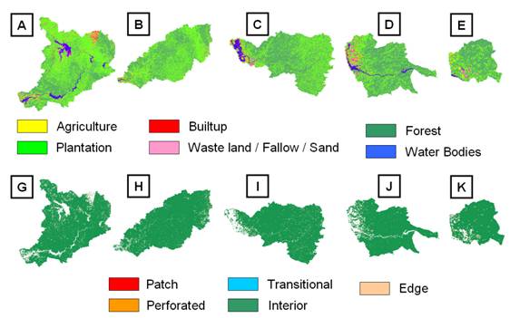
While the forest fragmentation map produced valuable information, it also helped to visualise the state of forest for tracking the trends and to identify the areas where forest restoration might prove appropriate to reduce the impact of forest fragmentation. Forest fragmentation also depends on the scale of analysis (window size) and various consequences of increasing the window size are reported in [15]. The measurements are also sensitive to pixel size. Nepstad et al., (1999a, 1999b) [18, 19] reported higher fragmentation when using finer grain maps over a fixed extent (window size) of tropical rain forest. Finer grain maps identify more nonforest area where forest cover is dominant but not exclusive. The strict criterion for interior forest is more difficult to satisfy over larger areas. Although knowledge of the feasible parameter space is not critical, there are geometric constraints [20]. For example, it is not possible to obtain a low value of Pff when Pf is large. Percolation theory applies strictly to maps resulting from random processes; hence, the critical values of Pf (0.4 and 0.6) are only approximate and may vary with actual pattern. As a practical matter, when Pf > 0.6, nonforest types generally appeared as “islands” on a forest background, and when Pf < 0.4, forests appeared as “islands” on a nonforest background.

There are five major west flowing rivers – Kali, Bedthi, Aginashini, Sharavathi and Venkatpura. Since LU in the catchment area of a river plays an important role in defining the course of the river, water quality and water retaining properties of the soil grains due to the presence of vegetation, the analysis was done for each watershed separately. LU map and forest fragmentation map of the five river basins are shown in Fig. 6 and statistics are given in table III. All the rivers are perennial since the catchment areas are mainly composed of interior forest. However, people have started converting forest patches for agricultural purposes. In addition, the dams present in the major rivers of the district have inundated large vegetation areas. These areas have silt deposit at the river beds and have been classified as sand / waste land. If the vegetative areas have been cleared, the water retaining capacity of the soil has decreased, triggering landslides in those areas. There is a immediate need to restore those vegetative by forestation to ensure that the soil is retained on the hill slopes and do not activate any downward movement of the hill tops.

Conclusion

The analysis showed that although the proportion of vegetation (natural forest and plantation which include – Acacea, Araca, Euclyptus, etc.) constitute major part of the LU in the district, recent field survey indicate many forest patches being used for agricultural activities. Conversions of land from forests to agriculture in undulating terrains have contributed to land slides, evident from the field data of landslides in the region. Hence, forest restoration is required to avoid erosion and prevent landslides.   

VI. Acknowledgment
This research was carried out with the financial assistance from ISRO-IISc Space Technology Cell. We thank NRSA, Hyderabad for providing IRS 1D data.

Fig. 6. LU in  the catchments of  five major river basins in Uttara Kannada district –  (A) Kali, (B) Bedthi, (C) Aginashini, (D) Sharavathi, (E) Venkatpura.
Forest fragmentation in  five river basins in Uttara Kannada district – (G) Kali, (H) Bedthi, (I) Aginashini, (J) Sharavathi, (K) Venkatpura.

Table III: LU Details of the five river basins

Classes	Agriculture		Builtup		Forest		Plantation		Waste land / Fallow / Sand		Water Bodies
AREA	Ha	%	Ha	%	Ha	%	Ha	%	Ha	%	Ha	%
Kali	13305	3.56	3176	0.85	127311	34	203491	54.4	11240	3	15023	4
Bedthi	5671	2	652.4	0.24	126532	46.3	136746	50	2616	0.96	1242	0.45
Aginashini	3654	2.68	673	0.49	72356	53	53604	39.3	1929	1.41	4323	3.17
Sharavathi	2537	3.13	607.7	0.75	49367	61	23794	29.4	2093	2.58	2627	3.24
Venkatpura	778	3.45	73	0.32	14491	64.3	6507	28.8	509	2.26	197.8	0.88

Table Iv: Forest Fragmentation Details of the five river basins

Classes	Patch		Transitional		Edge		Perforated		Interior
AREA	Ha	%	Ha	%	Ha	%	Ha	%	Ha	%
Kali	359	0.11	1085	0.33	4119	1.25	3027	0.92	321589	97.4
Bedthi	159	0.06	501	0.19	2462	0.94	1655	0.63	258209	98.18
Aginashini	70.8	0.06	234.6	0.19	1191	0.95	961	0.76	123265	98.05
Sharavathi	53	0.07	163.3	0.22	632.2	0.87	571.1	0.78	71465.8	98.05
Venkatpura	23.49	0.11	67.08	0.32	246.3	1.18	225	1.07	20379	97.32

REFERENCES

1. H. I. Cakir, and S. Khorram, “Pixel Level Fusion of Panchromatic and Multispectral Images Based on Correspondence Analysis,” Photogrammetric Engineering & Remote Sensing,vol. 74(2), pp. 183-192, 2008.
2. J. Nunez, X. Otazu, O. Fors, A. Prades, V. Pala, and R. Arbiol, “Multiresolution-Based Image Fusion with Additive Wavelet Decomposition,” IEEE Transactions of Geoscience and Remote Sensing, vol. 37(3), pp. 1204-1221, 1999.
3. J. L. Starck and F. Murtagh, “Image restoration with noise suppression using the wavelet transform,” Astron. Astrophys, vol. 228, pp. 342-350, 1994.
4. Venkatesh, Y.V., KumarRaja, S., 2003. On the classification of multispectral satellite images using the multilayer perceptron. Pattern Recognition, vol.  36, pp. 2161 – 2175.
5. B. V. Dasarathy (Editor), Nearest neighbor (NN) norms: NN pattern classification techniques, IEEE Computer Society Press, Los Alamitos, California, 1990.
6. P. J. Hardin, “Parametric and Nearest-neighbor methods for hybrid classification: A comparison of pixel assignment accuracy,” Photogrammetric Engineering & Remote Sensing, vol. 60, pp. 1439-1448, Dec, 1994.
7. R. P. Tucker, and J. F. Richards, “Global deforestation and the nineteenth century world economy,” Duke University Press, Durham, North Carolina, USA, 1983.
8. B. L. Turner, W. C. Clark, R. W. Kates, J. F. Richards, J. T. Mathews, and W. B. Meyer, “The Earth as transformed by human action,” Cambridge University Press, Cambridge, UK, 1990.
9. W. B. Meyer, and B. L. Turner, “Changes in land use and land cover: a global perspective,” Cambridge University Press, Cambridge, UK, 1994.
10. R. A. Houghton, “The worldwide extent of land-use change,” BioScience, vol. 44, pp. 305-313, 1994.
11. J. D. Hurd, E. H. Wilson, S. G. Lammey, and D. L. Civco, “Characterization of Forest Fragmentation and Urban Sprawl using time sequential Landsat Imagery,” In ASPRS 2001 Annual Convention, St. Louis, MO, 2001.
12. R. T. T. Forman, and M. Godron, “Landscape Ecology,” John Wiley, New York, 1986.
13. M. G. Turner, “Landscape ecology: the effect of pattern on process,” Annual Review of Ecology and Systematics, vol. 20, pp. 171-197, 1989.
14. S. A. Levin, “The problem of pattern and scale in ecology,” Ecology, vol. 73, pp. 1943-1967, 1992.
15. K., J. Riitters, R. O' Neill. Wickham, B. Jones, and E. Smith, “Global-scale patterns of forest fragmentation,” Conservation Ecology, vol. 4(2-3), 2000.
16. T. V. Ramachandra and A. V. Nagarathna, “Energetics in paddy cultivation in Uttara Kannada district,” Energy Conservation and Management, vol. 42( 2), pp. 131-155, 2001.
17. McFeeters, S. K., 1996. The use of normalized difference water index (NDWI) in the delineation of open water features, International Journal of Remote Sensing, 17(7): 1425–1432.
18. D. C. Nepstad, P. Lefebvre, and E. A. Davidson, “Positive feedbacks in the fire dynamic of closed canopy tropical forests,” Science, vol. 284, pp. 1832-1835, 1999a.
19. D. C. Nepstad, A. Verissimo, A. Alencar, C. Nobre, E. Lima, P. Lefebvre, P. Schlesinger, C. Potter, P. Moutinho, E. Mendoza, M. Cochrane, and V. Brooks, “Large-scale impoverishment of Amazonian forests by logging and fire,” Nature, vol. 98, pp. 505-508, 1999b.
20. R. V. O’Neill, C. T. Hunsaker, S. P. Timmins, B. L. Jackson, K. B. Jones, K. H. Ritters, and J. D. Wickham, “Scale problems in reporting landscape pattern at the regional scale,” Landscape Ecology, vol. 11, pp. 169-180, 1996.

Move to Annexure V

Photos