|
Results
Simulated data
Accuracy assessment of the abundance maps for 3 classes with small, medium and large variability obtained from VECLS algorithm with reference abundance maps is depicted in Table 5, 6 and 7 respectively. Fig.4, 5 and 6 shows the impact of intra-class variability on the accuracy of unmixing. Note that there are no pixels with abundances from 20% up to 70% in the abundance maps. The scatter in the relationship between predicted and actual class composition increases with an increase in the degree of intra-class spectral variation (from Fig.4 to 6 for each class), reducing the accuracy of the sub-pixel class composition estimates derived in Table 5. However, these accuracies are far better when compared to abundance estimation without endmember variability, also evident from Table 5.
The correlation and RMSE between predicted and actual/real/reference proportions with spatially degraded (down sampled) images are shown in Table 6 (at 50% of the original image size i.e. 50 x 50) and Table 7 (at 10% of the original image size i.e. 10 x 10). It is evident from these Tables that VECLS has an improved accuracy over CLS method. That is, the variability in endmembers has been accounted by the proposed algorithm than assuming single endmember per class. By degrading the images, it was observed that the accuracy comes down marginally and there is no drastic reduction. However, one important conclusion that can be drawn is that it is difficult to capture more variability with higher accuracy. Controlled variability and the effect of changing resolution resulted in two important findings: (i) As variability increases, the accuracy of classification decreases. In fact, the accuracy of sub-pixel fraction estimates linearly decreases with intra-class variability (Barducci & Mecocci, 2005; Settle, 2006).This is rational because higher the intra-class variability, more is the likelihood that the actual spectral characteristics of the endmembers in a pixel will deviate from the fixed endmembers. (ii) Down sampling of image pixels (from high to low resolution) affects the overall accuracy marginally with linear unmixing when a) the endmembers have been identified properly at each original image resolution with respect to the ground conditions and,b) the data fit well into the linear model.
Table 5 : Accuracy of prediction derived from low, medium and large variability data compared to absence of endmember variability (single spectra for each endmember) for 100 x 100 dimension images.
| Small variability |
| |
VECLS |
CLS (0 covariance) |
VECLS |
CLS (0 covariance) |
| Class |
Correlation coefficient (r) (p < 2.2e-16) |
RMSE |
| 1 |
0.9998 |
0.7332 |
0.0029 |
0.2312 |
| 2 |
0.9999 |
0.7403 |
0.0005 |
0.2077 |
| 3 |
0.9999 |
0.7406 |
0.0004 |
0.2088 |
| Medium variability |
| 1 |
0.9948 |
0.7155 |
0.0386 |
0.2506 |
| 2 |
0.9989 |
0.7380 |
0.0153 |
0.2104 |
| 3 |
0.9954 |
0.7321 |
0.0308 |
0.2181 |
| Large variability |
| 1 |
0.9851 |
0.7897 |
0.0563 |
0.2114 |
| 2 |
0.9968 |
0.7344 |
0.0259 |
0.2712 |
| 3 |
0.9850 |
0.8076 |
0.0561 |
0.1399 |
Table 6 : Accuracy of prediction derived from low, medium and large variability data compared to absence of endmember variability at half the original image dimension.
| Small variability |
| |
VECLS |
CLS (0 covariance) |
VECLS |
CLS (0 covariance) |
| Class |
Correlation coefficient (r) (p < 2.2e-16) |
RMSE |
| 1 |
0.9944 |
0.7105 |
0.0039 |
0.1732 |
| 2 |
0.9988 |
0.7211 |
0.0015 |
0.1223 |
| 3 |
0.9988 |
0.7213 |
0.0015 |
0.1221 |
| Medium variability |
| 1 |
0.9921 |
0.7341 |
0.0089 |
0.1022 |
| 2 |
0.9973 |
0.7241 |
0.0011 |
0.1210 |
| 3 |
0.9921 |
0.7222 |
0.0088 |
0.1289 |
| Large variability |
| 1 |
0.9821 |
0.7879 |
0.0673 |
0.0779 |
| 2 |
0.9933 |
0.7339 |
0.0079 |
0.1052 |
| 3 |
0.9841 |
0.8069 |
0.0601 |
0.0649 |
Table 7 : Accuracy of prediction derived from low, medium and large variability data compared to absence of endmember variability at one-tenth of the original image dimension.
| Small variability |
| |
VECLS |
CLS (0 covariance) |
VECLS |
CLS (0 covariance) |
| Class |
Correlation coefficient (r) (p < 2.2e-16) |
RMSE |
| 1 |
0.9911 |
0.7101 |
0.0029 |
0.2111 |
| 2 |
0.9985 |
0.7199 |
0.0009 |
0.2101 |
| 3 |
0.9983 |
0.7201 |
0.0011 |
0.2091 |
| Medium variability |
| 1 |
0.9889 |
0.7977 |
0.0005 |
0.2061 |
| 2 |
0.9890 |
0.7810 |
0.0004 |
0.2405 |
| 3 |
0.9900 |
0.7001 |
0.0414 |
0.2813 |
| Large variability |
| 1 |
0.9237 |
0.7297 |
0.1841 |
0.2417 |
| 2 |
0.9122 |
0.7544 |
0.1977 |
0.2106 |
| 3 |
0.9114 |
0.8076 |
0.1985 |
0.1917 |
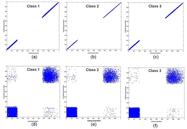
Fig. 4. The impact of small intra-class variability on the accuracy of unmixing using VECLS (a-c) and using CLS without variability (d-f).
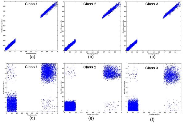
Fig. 5. The impact of medium intra-class variability on the accuracy of unmixing using VECLS (a-c) and using CLS without variability (d-f).
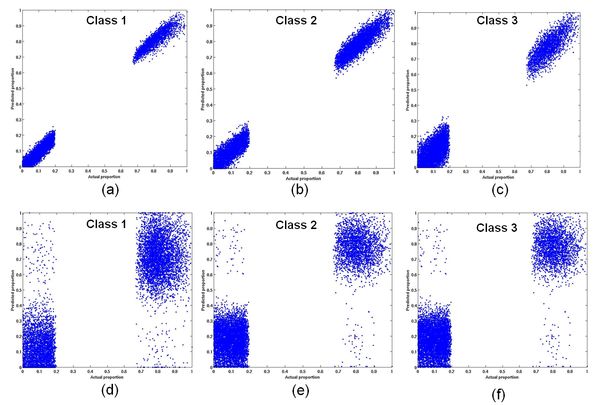
Fig. 6. The impact of large intra-class variability on the accuracy of unmixing using VECLS (a-c) and using CLS without variability (d-f).
Remote sensing data
The IKONOS, Landsat ETM+ and MODIS images were unmixed using VECLS method taking into account covariance due to variability in endmembers and later, subsequently assuming endmembers with zero covariance for comparison (Fig.7). The MODIS unmixed images are not shown in Fig. 7 due to space constraint. The obtained abundances were validated using correlation and RMSE as shown in Tables 8, 9 and 10.
Table 8 : Accuracy of prediction for IKONOS images for 2 and 3 classes with and without endmember variability
| IKONOS (4 m) |
| |
VECLS |
CLS (0 covariance) |
VECLS |
CLS (0 covariance) |
| 2 Class |
Correlation coefficient (r) (p < 2.2e-16) |
RMSE |
| vegetation |
0.9951 |
0.8122 |
0.0527 |
0.1745 |
| non-vegetation |
0.9751 |
0.8222 |
0.0751 |
0.1688 |
| |
| 3 Class |
Correlation coefficient (r) (p < 2.2e-16) |
RMSE |
| Urban |
0.9307 |
0.7998 |
0.0715 |
0.2173 |
| vegetation |
0.9461 |
0.7843 |
0.0602 |
0.2207 |
| Water |
0.9747 |
0.7678 |
0.0321 |
0.0302 |
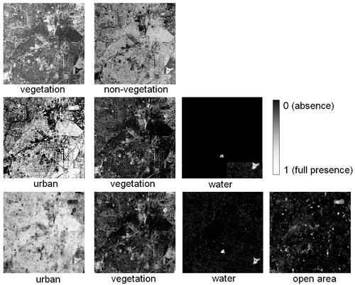
Fig. 7. Classified output for 2 classes (vegetation, non-vegetation), 3 classes (urban, vegetation and water) from IKONOS, and 4 classes (urban, vegetation, water and open area) from Landsat ETM+
Fig. 8, 9 and 10 indicates that, in general, abundances obtained from VECLS technique are much better than CLS method. For 2 and 3 classes, with decrease in the spatial resolution, the accuracy also decreases. However, this may not be always true when using Landsat and MODIS datain case of vegetation (Fig. 8) and in case of vegetation, water and open area for 4 classes (Fig. 10). The accuracy depends on the actual number of endmembers present in the image correlated to ground conditions and also the capability of the spectral bands to distinguish those objects.
Table 9 : Accuracy of prediction for Landsat images for 2, 3 and 4 classes with and without endmember variability
| Landsat (25 m) |
| |
VECLS |
CLS (0 covariance) |
VECLS |
CLS (0 covariance) |
| 2 Class |
Correlation coefficient (r) (p < 2.2e-16) |
RMSE |
| vegetation |
0.9307 |
0.7998 |
0.0744 |
0.2109 |
| non-vegetation |
0.9461 |
0.7843 |
0.0609 |
0.2346 |
| |
| 3 Class |
Correlation coefficient (r) (p < 2.2e-16) |
RMSE |
| urban |
0.8905 |
0.7290 |
0.1165 |
0.2846 |
| vegetation |
0.9104 |
0.7967 |
0.0935 |
0.2195 |
| water |
0.9214 |
0.7519 |
0.0827 |
0.2516 |
| |
| 4 Class |
Correlation coefficient (r) (p < 2.2e-16) |
RMSE |
| urban |
0.8413 |
0.6714 |
0.1424 |
0.3375 |
| vegetation |
0.8525 |
0.6385 |
0.1589 |
0.3787 |
| water |
0.8825 |
0.6192 |
0.1205 |
0.3926 |
| open area |
0.8161 |
0.6439 |
0.1749 |
0.3596 |
Table 10 : Accuracy of prediction for MODIS images for 2, 3 and 4 classes with and without endmember variability
| MODIS (250 m) |
| |
VECLS |
CLS (0 covariance) |
VECLS |
CLS (0 covariance) |
| 2 Class |
Correlation coefficient (r) (p < 2.2e-16) |
RMSE |
| vegetation |
0.9273 |
0.7761 |
0.0911 |
0.2389 |
| non-vegetation |
0.9137 |
0.7561 |
0.0855 |
0.2522 |
| |
| 3 Class |
Correlation coefficient (r) (p < 2.2e-16) |
RMSE |
| urban |
0.8621 |
0.7036 |
0.1490 |
0.3054 |
| vegetation |
0.8882 |
0.7055 |
0.1229 |
0.3003 |
| water |
0.8414 |
0.7165 |
0.1620 |
0.2946 |
| |
| 4 Class |
Correlation coefficient (r) (p < 2.2e-16) |
RMSE |
| urban |
0.8231 |
0.6606 |
0.1777 |
0.4470 |
| vegetation |
0.8731 |
0.6804 |
0.12093 |
0.3206 |
| water |
0.8930 |
0.6842 |
0.1142 |
0.3292 |
| open area |
0.7971 |
0.6492 |
0. 2105 |
0.3629 |
Also, with a very high spatial resolution data such as IKONOS with 4 m spatial resolution, LMM would not be always very useful. Ideally, in this case, we may get abundances as 1 or 0 since there are high chances that the intrinsic scale of objects on the ground may be of the order of 1 IKONOS MS pixel. On the other hand, LMM might work best for low spatial resolution and high spectral resolution (such as MODIS) as evident from Fig.10 for vegetation, water and open area classes. Since class separability depends on the number of spectral bands, so the separation between endmembers of different classes is important for obtaining higher accuracy. As also evident from simulated data analysis, increase in variability may reduce classification accuracy, but degrading the spatial resolution may not always decrease the accuracies of individual classes compared to accuracies obtained from classification of high spatial resolution data, provided a minimum residual error linear model with proper endmember selection is achieved. Urban class was identified with higher accuracy in IKONOS and Landsat bands compared to MODIS bands. Usually, urban areas have more heterogeneity with contrasting features and variability compared to other LC classes. Moreover, spatial extent of the urban objects are typically of high to medium spatial resolution pixel size, so Landsat data would be appropriate for urban land use / land cover types of studies while IKONOS data would be best for micro level urban studies.
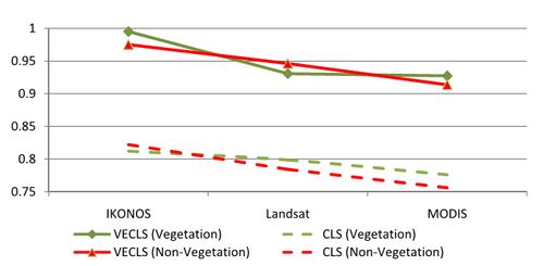
Fig. 8. Correlation between actual and predicted proportion for 2 classes with changing spatial resolutions
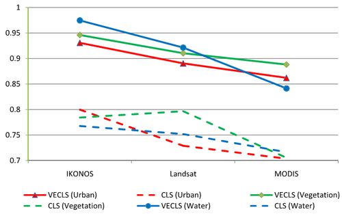
Fig. 9. Correlation between actual and predicted proportion for 3 classes with different sensor data
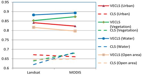
Fig. 10. Correlation between actual and predicted proportion for 4 classes with different sensor data.
|
