|
Data and Methods
A major problem involved in analysing the quality of fractional estimation methods is the fact that ground truth information about the real abundances of materials at sub-pixel levels is difficult to obtain in real scenarios. Therefore, simulated dataset were used to illustrate and explore the effect of class spectral variability on sub-pixel class composition estimation in a controlled analysis as single class is difficult to be adequately represented by a unique endmember which remains an implicit assumption in unmixing, (Asner et al., 1998; Song & Woodcock, 2003; Townshend et al., 1992). Advantages are that the exact endmember fractions are known and in addition, the non-linear interactions of photons among endmembers (Kumar et al., 2012) do not exist, simplifying the problem and allowing better understanding of the impact of endmember variability.
With real time RS data, the impacts of class spectral variation on sub-pixel class composition estimation has been illustrated by addressing the spatial variability of LC components as a combination of endmembers, and spectral variability has been addressed by allowing the number and type of endmembers to vary from pixel to pixel.The entire methodology is summarized in steps as follows:
Step-1: Geo-correction of RS data.
Step-2: Decide the number of LCclasses.
Step-3: Derive individual endmembers from the image.
Step-4: Correlate endmembers to ground conditions (LC classes).
Step-5: Select many instances of endmembers to account for the statistical variability.
Step-6: Represent each class by its mean and variance-covariance matrix.
Step-7: Apply VECLS algorithm.
Step-8: Obtain abundance map for each class.
Step-9: Validate abundance maps with ground truths using correlation, RMSE, and BDF plots.
1. Simulated data
Spectral libraries of three minerals – alunite (endmember1), buddingtonite (endmember2), and kaolinite (endmember3) available at http://speclib.jpl.nasa.gov/ were used to generatesimulated data, which comprisesof three classes. Also, to accommodate for the dimensionality constraint in unmixing (Settle and Drake, 1993), four simulated spectral wavebands of 100 x 100 dimensions were considered. The spectral responses of each class in each waveband were varied (from small to medium to large) in separate experiments to illustrate the impacts of differences in intra-class variation.
Initially, means of different classes (Table 2) were taken to define the class endmember spectra and thenused to generate abundance maps for validating the output of VECLS algorithm.Here, each pixel was obtained from a LMM and the endmembers of each category was drawn from a Gaussian distribution where the mean of each endmember can be set and the variability can be controlled.
Table 2: Mean endmembers and spread around the mean for small, medium and large variability.
| Class |
Mean endmember in Band 1 |
Mean endmember in Band 2 |
Mean endmember in Band 3 |
Mean endmember in Band 4 |
Spread to control variability |
| 1 |
142 |
136 |
135 |
74 |
0.001 |
| 2 |
81 |
69 |
56 |
203 |
7 |
| 3 |
140 |
132 |
96 |
7 |
20 |
Artificial bands are assumed to be of the form: mean + Gaussian perturbation given by covariance, i.e.,
endmember1 = mean1 + random perturbation;
endmember2 = mean2 + random perturbation;
endmember3 = mean3 + random perturbation;
where, random perturbation is a Gaussian random variable of 0 mean and specific variance. So,
artificial band = abundance1 × endmember1 + abundance2 × endmenber2 + abundance3 × endmenber3 ..............(27)
The statistical properties of each simulated band are given in Table 3. A multitude of LMMs were applied with different endmembers and a series of sub-pixel class composition estimates were obtained for a pixel of given spectral response. The bands were spatially degraded to 50 x 50 dimension (half the spatial resolution of the original image) and to 10 x 10 dimension (one tenth of the original image dimension) to study the impact of endmember variability at different spatial scales. In this way, we could analyse not only the impact of variable endmembers, but also the impact of variability in endmembers with respect to change in spatial resolutions. In another set of experiments, covariance of all the endmembers were made zero, i.e. assuming each endmember is being represented by only one spectrally pure pixel and there is no variation within an endmember. The idea behind doing this was to compare the performance of the algorithm in two complementary cases, namely, when the endmembershave (i) variability, (ii) no variability.
Table 3: Statistical properties of the simulated data
| Small variability |
| Bands |
Minimum |
Maximum |
Range |
Mean |
Variance |
Variation coefficient (%) |
| 1 |
80.99 |
142.00 |
61.02 |
124.72 |
353.95 |
15.09 |
| 2 |
69.03 |
136.03 |
67.01 |
116.51 |
419.93 |
17.59 |
| 3 |
55.96 |
134.95 |
78.99 |
102.34 |
548.70 |
22.89 |
| 4 |
7.02 |
202.99 |
195.97 |
90.46 |
2652.17 |
56.93 |
| Medium variability |
| 1 |
76.42 |
149.98 |
73.56 |
124.71 |
358.24 |
15.18 |
| 2 |
65.08 |
141.18 |
76.09 |
116.50 |
424.60 |
17.69 |
| 3 |
50.49 |
139.45 |
89.26 |
102.33 |
553.69 |
22.99 |
| 4 |
5.12 |
205.75 |
200.63 |
90.47 |
2657.12 |
56.98 |
| Large variability |
| 1 |
69.36 |
153.70 |
84.34 |
124.78 |
366.32 |
15.34 |
| 2 |
59.84 |
149.93 |
90.09 |
116.60 |
435.10 |
17.89 |
| 3 |
44.94 |
147.47 |
102.54 |
102.43 |
560.94 |
23.12 |
| 4 |
2.87 |
207.81 |
204.94 |
90.33 |
2661.18 |
57.11 |
It was ensured that there are instances of 100% class proportions in the three abundance maps generated using simulated data. These pixels were then mapped to the original bands and corresponding pixel values were extracted as endmembers. User defined means and spread around the mean could be incorporated into the simulated data and hence, the endmembers in the 4 bands were cross verified with the class means. Endmembers were also visualised using scatterplots (Fig.2) which shows location of classes defined by the means in simulated data with small, medium and large variability, where each class occupies an area of the feature space. It is obvious that any one point in the feature space can be associated with a variety of class compositions.
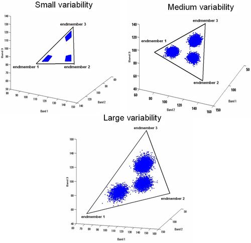
Fig. 2. Endmember locations defined by the extreme pixels in small, medium and large variability datasets for 3 classes.
Remote sensing data
The VECLS algorithm was assessed for its performance in unmixing mixed pixels of various spatial and spectral resolutions. Initially, IKONOS 4 bands MS data of 4 m spatial resolution were fused with IKONOS 1 m Panchromatic (PAN) band using Smoothing Filter based Intensity Modulation (SFIM) fusion (Liu, 2000) based on comparative analysis of the image fusion results (Kumar et al., 2009; 2011). Training pixels were taken from the False Colour Composite (FCC) and supervised classification using Maximum Likelihood Classifier (MLC) (Duda et al., 2000; Richards and Jia, 2006; Zheng et al., 2005) was performed on the fused data (1 m) to classify the image into 2 classes (vegetation, non-vegetation), 3 classes (urban, vegetation and water) and 4 classes (urban, vegetation, water and open area). The overall accuracy of the classified imageswere 98% (2 classes), 96% (3 classes) and 93% (4 classes) respectively. These classified maps were used as references to validate the sub-pixel maps obtained using VECLS and CLS. A series of experiments with varying resolutions and varying classes (2, 3 and 4) were carried out to illustrate the performance of the proposed algorithm. The details of the data (IKONOS PAN (1 m) and MS (4 m), Landsat ETM+ MS (25 m) and MODIS 7 bands (250 m)) used are provided in Table 4.
Table 4 : Remote sensing datasets used for validating VECLS algorithm
| Data |
Spectral bands |
Spatial resolution |
Dimension |
2 classes |
3 classes |
4 classes |
| IKONOS PAN and MS fused |
4 |
1 m |
8000 x 8000 |
vegetation, non-vegetation |
urban,
vegetation,water |
urban,
vegetation, water,
open area |
| IKONOS |
4 |
4 m |
2000 x 2000 |
vegetation, non-vegetation |
urban,
vegetation,water |
--- |
| Landsat |
6 |
30 m resampled to 25 m |
320 x 320 |
vegetation, non-vegetation |
urban,
vegetation,water |
urban,
vegetation,water,
open area |
| MODIS |
7 |
250 m |
32 x 32 |
vegetation, non-vegetation |
urban,
vegetation,water |
urban,
vegetation,water,
open area |
The study area (Fig. 3) is a part of Bangalore City, India which is highly urbanised with considerable spectral variation (for example due to buildings with concrete roofs, tiled roofs, asbestos, asphalt, etc.) that exhibit high degrees of spectral heterogeneity on fine scales. The scene has dense buildings, bus stand, railway station, tarred roads with flyovers, parks, race course and lakes. There are few open areas (such as playground, walk ways and vacant land). This scene was appropriate to judge the performance of VECLS with highly contrasting and heterogeneous features at different spatial resolutions.We had little prior knowledge of the appropriate spatial scale for interpreting the fractions generated for an urban area.Hence, varying the spatial scale allowed us to investigate the impact of scales based on size of sampling unit, as well as to consider how confidentare the estimates of LC fractions that might vary with spatial scale.
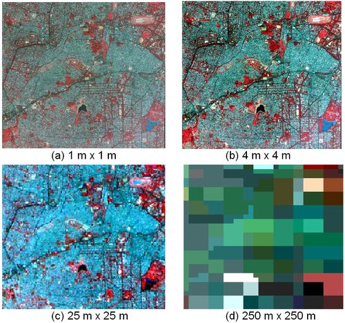
Fig. 3. False Colour Composite of the study area from (a) IKONOS (PAN and Multispectral fused), (b) IKONOS Multispectral, (c) Landsat ETM+ and (d) MODIS
Endmembers were extracted from IKONOS MS, Landsat and MODIS data using N-FINDRalgorithm (Boardman, 1995).The advantage of image endmembers is that they can be collected at the same scale as the image, therefore,endmembers are easier to associate with image features (Rashed et al., 2003) but have some associated error, which varies with the scale of the measurement used and the scale of intrinsic spatial variation (Settle, 2006).The N-FINDR algorithm is briefly given below.
- Let N denote the number of classes or endmembers to be identified.
- Perform a principal component analysis (PCA)-decomposition of the data and reduce the dimension of the data to N - 1. In what follows, we assume that the data are transformed to N - 1 dimension PCA space.
- Pick N pixels from the set and compute the simplex volume generated by the spectra of the N pixels. The volume of the simplex is proportional to
 (28) (28)
- Replace each endmember with the spectrum of each pixel in the data set and recompute the simplex volume. If the volume increases, the spectrum of the new pixel is retained as a potential endmember.
As the endmembers are at the extreme points of the convex hull, the N-FINDR algorithm tries to find out those pixels whose convex hull generated by their spectrum contains the spectra of all theother pixels achieved by maximising the volume of the simplex (convex hull). These steps are executed iteratively considering all the pixels and the final set of spectra retained are taken to be the endmembers(Winter, 1999).
These endmembers were also identified in the three FCCs and individual spectral bands of all the sensor data. Many instances of similar endmembers per class were chosen from the FCC and the scatterplots, and were incorporated into the VECLS algorithm. VECLS was applied on each dataset to obtain the abundance maps for 2, 3 and 4 classes. Since IKONOS has only 4 spectral bands, only 3 target classes could be used due to dimensionality constraints. The covariance of all the endmembers were also assumed zero to assess the performance of the algorithm in the absence of variability. This would give the relative benefits of the proposed method and highlight the advantages of considering variability in endmembers. |
