Introduction

Urban areas are currently among the most rapidly changing land cover (LC) types on the Earth. Urban cities are the loci of human population and activities, and are therefore sites of significant natural resource transformation (Lambin et al., 2001). Remote sensing (RS) has been widely used to provide a timely and synoptic view of urban LC (Kumar et al., 2011a;Yang and Lo, 2002).More often than not, the accuracy of urban LC mapping is limited by the presence of mixed pixels (Kumar et al., 2008). Deriving accurate, quantitative measures over urban area remains a fundamental research challenge due to the great spatial and spectral variability of the materials (Forster, 1985; Lu & Weng, 2004; Xian & Crane, 2005).In highly variable scenes, spatial heterogeneity (in the types and conditions) of endmembersof urban surface materials is problematic at multiple spatial scales, resulting in a high percentage of mixed pixels in most moderate to low spatial resolution imagery and occasionally, even limiting the utility of high spatial resolution imagery (Myint et al., 2004; Small, 2005; Somers et al., 2011).

There are two principal approaches to retrieve information on LC from multispectral (MS) satellite images. The most common approach to characterise LC from RS data is hard classification; assigning all pixels in the image to mutually exclusive classes such as built-up, water, vegetation, etc. (Carlson & Sanchez-Azofeifa, 1999; Kumar et al., 2011b; Powell et al., 2007) generating a thematic map at the resolution of the bands. This approach is problematic for several reasons – firstly, most urban LC classes are not spectrally distinct resulting in considerable confusion between classes (Small, 2005). Secondly, physical composition of the classes may vary due to different building materials and different construction practices and therefore cross regional comparisons between urban areas are limited (Small, 2005).This method depends on the assumption that two signals corresponding to one cover type are much more similar to each other than the two signals from different cover types (Settle, 2006). Another approach is linear unmixing – the linear mixture model (LMM), which allows a number of different LC types to be present, each contributing a fraction of its (unique, fixed) spectrum where fraction corresponds to the area occupied by that LC type which is obtained by inverting the model to produce estimates of those fractional abundances. The spectral signature (endmember) for each class may be obtained from the image itself (Bateson et al., 2000;Boardman, 1995; Kumar et al., 2008;Kumar et al., 2012;Plaza et al., 2004; Settle, 2006;Winter and Winter, 2000) or from libraries of reference spectra(Dennison and Roberts, 2003). The selectionof endmembers involves identifying both the number and type of endmembers and their corresponding spectral signatures. Various approaches for selecting endmembers have been proposed (refer Plaza et al., 2004, 2005; Martinez et al., 2006; Miao and Qi, 2007;Dobigeon et al., 2009, etc.).  However, the use of fixed endmember spectra does not take into account the variation in endmember spectral signatures caused by differential illumination conditions,spatial and temporal variability in the scene components resulting in significant fraction estimate errors.

The pixel-to-pixel variability in an image can be explained in two different ways as described by Settle (2006).Firstly, the main distinction is between pixels of different LC types, with further variation coming from within-class variability. Secondly, there is no within-class variability, but the variations in reflectance within the pixels arise from pixel-to-pixel variations in the fractional coverage. This could lead us to infer that if the intrinsic scale of the pixel is smaller than the changes in LC type, hard classification is justified, while unmixing is appropriate when the case is reverse, given the underlying class membership model. The fundamental reason for this variability is the issue of scale and hence toggling between the two models for addressing the variability in surface reflectance may not be appropriate. The phenomenon of variability is prevalent at a fine scale andit is unreasonable to ignore the effect of variability in pure LC classes at sufficiently high resolution while observing the same at a moderate or coarse resolution(Settle, 2006). Standard LMM assumes a fixed number of representative endmembers and the entire image is modeled in terms of those spectral components. However, urban environments are particularly difficult to model because a single endmember cannot account for considerable spectral variation within a class as they exhibit high degrees of spectral heterogeneity on fine scales. The procedure is limited because the selected endmember spectra may not effectively model all the elements in the image, or a pixel may be modeled by endmembers that do not actually correspond to the materials located in its field of view and result in decreased accuracy of the estimated fractions (Sabol et al., 1992). Thus, for each pixel, it may sometimes be more appropriate to recognise that a distribution of possible coverage may be derived for each class. The width of this distribution is a function of the degree of intra-class spectral variation (variability within the endmember class)present and will impact on the use of the sub-pixel classification output.

Various attempts have been made to address endmember variability.Somers et al., (2011) presented a detailed review of the available methods and results of endmember variability reduction in spectral mixture analysis based on the hypothesized five principleswhich arereviewed at the end of Section 3 (after the conceptual framework of VECLS algorithm).In recent times, numerous solutions (Somers et al., 2010a, 2010b) to account endmember variability have been proposed including the hierarchical Multiple Endmember Spectral Mixture Analysis (MESMA,Roberts et al., 1998) applied to map urban LC in Bonn, Germany, with a Hymap (126 spectral bands) and 4 levels of classification using 1521 endmembers obtained using EAR, MASA and COB (Franke et al., 2009). MESMA was also applied on Landsat ETM+ with four endmembers (vegetation, impervious surface, soil and water) for Manaus, Brazil (Powell et al., 2007). Foody and Doan (2007) reported the impact of intra-class spectral variability on the estimation of sub-pixel LC class composition concluding that class variation has an impact on the accuracy of sub-pixel class composition estimation, as it violates the assumption that a class can be represented by a single endmember. Settle (2006) attempted to derive an improved representation of error term in the mixture model, taking account of the variability of the endmember spectra and of sub-pixel variation in fraction abundance of surface cover. Song (2005) proposed a Bayesian spectral mixture analysis (BSMA) model to understand the impact of endmember variability on the deviation of sub-pixel vegetation fractions in an urban environment. This approach is similar to iterative mixture analysis, i.e. each pixel is unmixed with randomly selected combinations of endmember signatures, represented by probability density functions. BSMAaccounts the probabilities of spectral signatures instead of assuming equal probabilities for all endmembers. Bateson et al., (2000) constructed endmember bundles to produce minimum and maximum fraction images bounding the correct cover fractions and specifying error due to endmember variability.Recently, a pre-screened and normalised MESMA which includes a new endmember selection strategy and an integration of the normalised spectral mixture analysis (NSMA) and MESMA for estimating impervious surface area fraction was proposed by Yang et al., (2010). The methods proposed above are different in their approaches, underlying principles and assumptions. They have been tested on different datasets and there is no proper guideline as to which method and spatial resolution would be most suitable for optical RS data for a regional level urban area classification while taking into account the intra and inter class variabilityi.e. similarity among endmember classes (Zhang et al., 2006).

Here, we propose a novel technique– variable endmember constrained least square (VECLS) for addressing the endmember variability in an image. The methodology for classification allows the signals within a class to vary from pixel to pixel about a mean spectrum. Each class is then represented by the mean and by a variance-covariance matrix that captures the statistical variability around the mean, and allocation decisions are based on a modified form of statistical pattern matching. Many instances of a particular endmember are chosen from the image to take into account its variability. This inter-class variance is accounted by constructing a covariance matrix that varies around the selected endmember mean. The algorithm is first applied on a computer simulated dataset with 4 bands and 3 classes having small, medium and large variability in the endmember’s spread. The technique is then tested on real datasets acquired from IKONOS, Landsat ETM+ and MODIS sensors taking 2, 3 and 4 classes. The method is compared with a situation when there are no variances in the endmembers i.e. covariance within an endmember is zero. The results are validated with a high resolution classified map using correlation, root mean square error (RMSE), and bidirectional function (BDF) plots.The overall methodology is as depicted in Fig. 1.

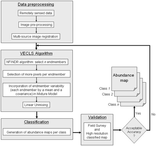
Fig. 1. Overall methodology flow diagram

The paper is organised as follows. Section 2 discusses the general linear model and the framework for VECLS algorithmis described in section 3. Section 4 presents data and methods, followed by results and discussion in section 5 and 6 respectively, with concluding remarks in section 7.