Landscape refers to a portion of heterogeneous territory composed of sets of interacting ecosystems and is characterized essentially by its dynamics that are partly governed by human activities (Ramachandra et al., 2012a). Human induced land use and land cover (LULC) changes have been the major drivers for the changes in local and global environments. Analyses of changes in land uses provide a historical perspective of land use and give an opportunity to assess the spatial patterns, correlation, trends, rate and impacts of the change, which would help in better regional planning and good governance of the region (Bhatta et al., 2010, Ramachandra, et al., 2012a, Ramachandra et al., 2012b).
Humans are influencing the forested landscape through many interventions fragmenting it into patches. Fragmentation is the breaking up of a landscape, habitat, ecosystems, or land use types into smaller parts (Forman, 1995 &1997), which results in the decreased size of the continuous landscape and lost connectivity between populations and the similar ecosystems (Griffiths et al. 2000).
Forest fragmentation is a process which results in loss of biodiversity and natural forest ecosystems through human influence.Fragmentationsof landscape have been quantified by change in spatial characteristics and configuration of remaining patches (Saunders et al. 1987). Various ecological effect of forest fragmentationsare loss of species populations, increased isolation of remnant populations, inbreeding (Laurance et al. 1998, Boyle 2001), enhanced human-animal conflicts, decline in ecosystem goods and services, etc.This necessitates understanding of the causes of forest and habitat fragmentations, in order to evolve effective management strategies for conservation.
Remote sensing (RS) data acquired through space borne sensors available post 70’s at regular intervalscan be used as one of the major tools to understand LULC dynamics and quantify the extent of forest fragmentation (Gustafson 1998; Turner & Gardner 1991). Remotely sensed(RS) data in conjunction with geographic information systems have been successfully utilized to quantify forest loss as well as forest fragmentation (Jha et al., 2005).Temporal analysis of the spatial data provides an idea of the extent of changes happening in the landscape. Land use details derived from temporal RS data offer potential for assessing the changes in land uses, forest fragmentation and its impact on ecology and biodiversity (Ramachandra et al., 2011). Categorization and understanding of forest fragmentation using spatial data (RS data) provides a picture of the degree and extent of fragmentation, which are useful for conservation of the affected habitat fragments (O’Neill et al.,1997).
Numerous measures of forest fragmentation and forest connectivity using spatial data include average forest patch size, mean forest patch density, number of forest patches, forest patchiness, forest continuity, and proportion of forest in the largest forest patch (Vogelmann, 1995; Trani and Giles, 1999; Wickham et al.1999). Quantification of pf and pff has effectively helped in assessing the process of fragmentation (Ramachandra et al., 2011). This section assesses the LULC dynamics in Shimoga and examines the extent of forest fragmentation in Shimogalandscape.
Material
The spatial data acquired from Landsat Series Multispectral sensor (57.5m) and thematic mapper (28.5m) IRS LISS III sensors for the period 1979 to 2010 were downloaded from public domain as indicated in Table 1. Survey of India (SOI) topographic maps of 1:50000 and 1:250000 scales were used to generate base layers of city boundary, etc.
Table 1: Data used in the Analysis
| DATA |
Year |
Purpose |
| Landsat Series Multispectral sensor(57.5m) |
1973 |
Land cover, Land use analysis and Fragmentation analysis |
| Landsat Series Thematic mapper (28.5m) |
1990 |
Land cover, Land use analysis
and Fragmentation analysis |
| IRS LISS III |
2001, 2010 |
Land cover, Land use analysis
and Fragmentation analysis |
| Survey of India (SOI) toposheets of 1:50000 and 1:250000 scales |
|
To Generate boundary and Base layer maps. |
| Field visit data –captured using GPS |
|
For geo-correcting and generating validation dataset |
| Google earth and Bhuvan |
|
For digitizing various attribute data and as validation input |
METHOD
Landscape Dynamics: Assessment of landscape dynamics involved (i) land use and land cover assessment considering temporal remote sensing data, (ii) quantification of fragmentation of natural forests, (iii) assessment of extent of fragmentation due to encroachment (and subsequent changes in land uses).The procedure followed to assess landscape dynamics is outlined in Figure 1.
The spatio-temporal changes in land use and land cover (LULC) of the study region were studied using temporal RS data with geospatial techniques. Spatial data acquired through space borne sensors at regular intervals since 1970’s aid in monitoring of large areas and enablethe change analyses at local, regional scales over time (Wilkie and finn, 1996). Remote sensing data along with field data collection usingpre-calibrated GPS (Global Positioning System) help in the effective land use analysis (Ramachandra et al., 2012a).
The remote sensing data obtained were geo-referenced, rectified and cropped pertaining to the study area. Geo-registration of remote sensing data (Landsat data) has been done using ground control points collected from the field using GPS and also from known points (such as road intersections, etc.) collected from geo-referenced topographic maps published by the Survey of India.
Remote sensing data requires preprocessing like atmospheric correction and geometric correction in order to enable correct area measurements, precise localization and multi-source data integration (Ramachandra and Bharath, 2012b, Buiten, 1994). Geometric correction is the process of referencing an image to a geographic location (real earth surface positions) using GCP’s (ground control points). GCP’s were collected from the toposheet (SOI) as well as from field using hand held pre-calibrated GPS. This helped in geometrically correcting the distorted remote sensing data.Landsat satellite 1973 data have a spatial resolution of 57.5 m x 57.5 m (nominal resolution) were resampled to 28.5m comparable to the 1989 - 2010 data which are 28.5 m x 28.5 m (nominal resolution).
1. LAND COVER ANALYSIS:
Spatiotemporal change detection process involves determining the changes associated with LULC properties with reference to geo-registered multi temporal remote sensing data.
The monitoring of land cover involves the computation of vegetation indices. The land cover analysis was done using NDVI (Normalized Difference Vegetation Index). Among all techniques of land cover mapping, NDVI is most widely accepted and applied (Zhanget al., 2007, Jensen et al., 1982, Nelson et al,. 1983).Calculation of NDVI for multi-temporal data is advantageous in areas where vegetation changes rapidly. The capability of capturing changes in land cover and extracting the change information from satellite data requires effective and automated change detection techniques (Ramachandra et al., 2009, Roy et al., 2002). NDVI is calculated by using visible Red and NIR bands of the data reflected by vegetation. Healthy vegetation absorbs most of the visible light that hits it, and reflects a large portion of the near-infrared light. Sparse vegetation reflects more visible light and less near-infrared light. NDVI for a given pixel always results in a number that ranges from -1 to (+1), using Equation1
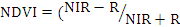 ) … (1)
2. LAND USE ANALYSIS:
This involvedi) generation of False Color Composite (FCC) of remote sensing data (bands – green, red and NIR). This helped in locating heterogeneous patches in the landscape ii) selection of training polygons (these correspond to heterogeneous patches in FCC) covering 15% of the study area and uniformly distributed over the entire study area, iii) loading these training polygons co-ordinates into pre-calibrated GPS, iv) collection of the corresponding attribute data (land use types) for these polygons from the field. GPS helped in locating respective training polygons in the field, v) supplementing this information with Google Earth vi) 60% of the training data has been used for classification, while the balance is used for validation or accuracy assessment.
The land use analysis was carried out with training data using supervised classification technique based on Gaussian Maximum Likelihood algorithm. The supervised classification approach preserves the basic land use characteristics through statistical classification techniques using a number of well-distributed training pixels. Gaussian Maximum Likelihood classifier (GMLC) is appropriate and efficient technique based on “ground truth” information for classifier learning. Supervised training areas are located in regions of homogeneous cover type. All spectral classes in the scene are represented in the various subareas and then clustered independently to determine their identity. The following classes of land use were examined: built-up, water, cropland, open space or barren land, and forest. Such quantitative assessments, will lead to a deeper and more robust understanding of land-use changesforan appropriate policy intervention. GRASS GIS (Geographical Analysis Support System), a free and open source software having the robust support for processing both vector and raster files accessible at http://wgbis.ces.iisc.ac.in/grass/index.phpis used for the analysis.
Accuracy assessments decide the quality of the information derived from remotely sensed data. The accuracy assessment is the process of measuring the spectral classification inaccuracies by a set of reference pixels.These test samples are then used to create error matrix (also referred as confusion matrix),kappa (κ) statistics and producer's and user's accuracies to assess the classification accuracies. Kappais an accuracy statistic that permits us to compare two or more matrices andweighs cells in error matrix according to the magnitude of misclassification.
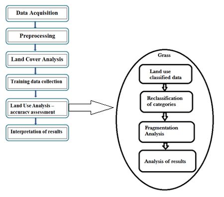
Figure 1: LULC and fragmentation analysis
3. FRAGMENTATION ANALYSIS:
Forest fragmentation analysis was done to evaluate the extent of fragmentation through quantification of - patch, transitional, edge, perforated, and interior forests using temporal classified land use data of Shimoga district.
Forest fragmentation statistics pf and pffis computed using fixed-area kernel (3x3) considering the current pixel and its neighborhood (Ritters et al., 2000, Ramachandra et al., 2011). The result is stored at the location of the center pixel. Forest fragmentation category at pixel level is computed through Pf (the ratio of pixels that are forested tothe total non-water pixels in the window) and Pff(the proportion of all adjacent (cardinal directions only) pixel pairs that include at least one forest pixel, for which both pixels are forested). Pff estimates the conditional probability that given a pixel of forest, its neighbour is also forest. Based on the knowledge of Pf and Pff,six fragmentation categories derived (Figure 2) are (i) interior, when Pf= 1.0; (ii) patch, when Pf< 0.4; (iii) transitional, when 0.4 < Pf< 0.6; (iv) edge, when Pf> 0.6 and Pf– Pff> 0; (v) perforated, when Pf> 0.6 and Pf – Pff < 0, and (vi) undetermined, when Pf> 0.6 and Pf= Pff.
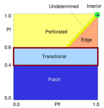
Figure 2: Forest Fragmentation using PF and PFF
RESULTS
Land cover analysis: Land cover analysis through NDVI shows the percentage of area under vegetation and non-vegetation. NDVI is based on the principle of spectral difference based on strong vegetation absorbance in the red and strong reflectance in the near-infrared part of the spectrum. Figure 3 and Table 2 illustrates the spatio-temporal changes in the land cover of the region, which highlight the decline of vegetation cover from 96.57 (1973) to 91.72%.
Table2: Extent of vegetation cover during 1973, 1990, 2002 and 2012
| Land Cover (%) |
| |
Vegetation |
Non-Vegetation |
| 1973 |
96.57 |
3.43 |
| 1990 |
96.43 |
3.57 |
| 2002 |
93.84 |
6.16 |
| 2012 |
91.72 |
8.28 |
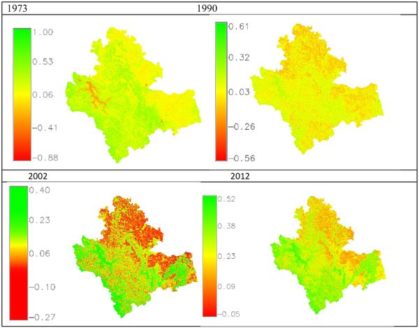
Figure 3: Vegetation dynamics in Shimoga
Land use analysis: Figure 4highlight changes in land uses at landscape level during 1973 to 2012. Table 3 illustrates the changes in land uses: built-up increased from 0.63% (1973) to 2.32% (2012) and forest vegetation decreased from 43.83% (1973) to 22.33% (2012). The results highlight conversion of forests to agricultures, industrial and cascaded developmental activities acted as major driving forces of degradation.Table 4 listsKappa statistics and overall accuracy.
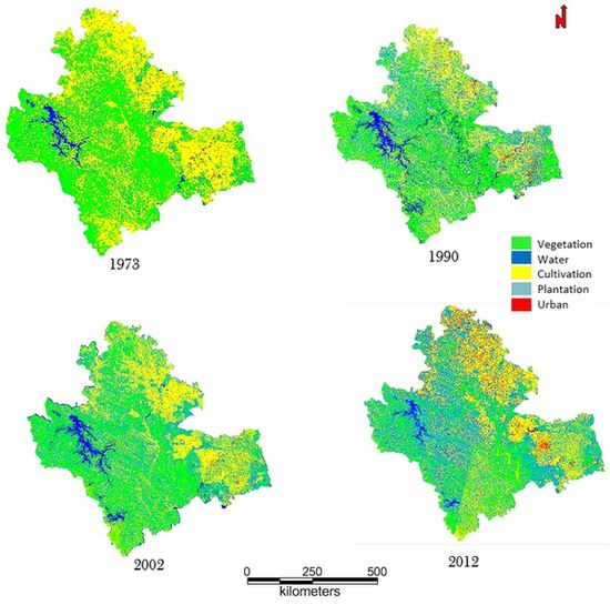
Figure 4. Land usechanges during 1973 to 2012 in Shimoga
Table3: Land use statistics
| Land use categories (%) |
| Years |
Urban |
Vegetation |
Water |
Cultivation and open area |
Plantation |
| 1973 |
0.63 |
43.83 |
1.91 |
44.14 |
9.46 |
| 1990 |
0.74 |
39.90 |
4.53 |
29.68 |
25.15 |
| 2002 |
1.08 |
37.78 |
4.57 |
30.21 |
26.36 |
| 2012 |
2.32 |
22.33 |
6.09 |
34.56 |
34.69 |
Table4: Kappa and overall accuracy
| Year |
Kappa coefficient |
Overall accuracy (%) |
| 1973 |
0.82 |
74.68 |
| 1990 |
0.89 |
86.31 |
| 2002 |
0.83 |
92.23 |
| 2012 |
0.91 |
91.48 |
Fragmentation analysis
Land use data (classified data with 4 classes) were used as input to the fragmentation analysis and the analysis was done at district and division levels. Figure 5illustrates the extent of forest fragmentations while Table 5 provides the summary statistics.
Table 5: Extent of forest fragmentation during 1973 to 2012
| Type of fragments |
1973 |
1990 |
2001 |
2012 |
| Patch |
3.95 |
5.00 |
3.31 |
2.05 |
| Transitional |
6.65 |
8.91 |
6.08 |
3.72 |
| Edge |
1.30 |
1.93 |
0.94 |
0.98 |
| Perforated |
12.79 |
9.89 |
15.73 |
8.19 |
| Interior |
18.55 |
14.01 |
9.37 |
6.88 |
| Undetermined/other category |
56.76 |
60.26 |
64.56 |
78.17 |
Applying forest fragmentation analysisto a time series of land use data provided a quantitative assessment of the pattern and trends in forest fragmentation. The analysis indicated that domination of forests receded during post 90’s with the formation of patch and edge forest in all 3 divisions. Land use changes from forests to non-forests with intensified human interference had been very high especially in Bhadravathi division. Interior forest decreased by 12% during 4 decades.
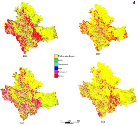
Figure 5: Fragmentation of forests in Shimoga
Forests in Shimoga district are administered through three divisions – Shimoga, Bhadravathi and Sagar.The quantification of extent of forest fragmentation has been done division-wise for the past four decades to enable the respective division administration to undertake appropriate forest restoration measures to minimize fragmentation of ecologically important ecosystems. Figure 6 illustrates spatially the extent of forest fragmentation in Shimoga. Similarly Figures 7 and 8 depicts the extent of fragmentation in Bhadravathi and Sagar divisions respectively.
The extent of interior forests ranges from 12.91 (Shimoga) followed by 4.76 (Sagar) and 3.79 % (Bhadravathi). During the last four decades the interior forest declined from 22.9 (1973) to 13 % (2012) in Shimoga, and 15.90 (1973) to 4.76% (2012) in Sagar, and 4.10 (1973) to 3.79 % (2012) in Bhadravathi divisions emphasizing the need for an immediate eco-restoration measures to arrest fragmentation and consequent impacts.
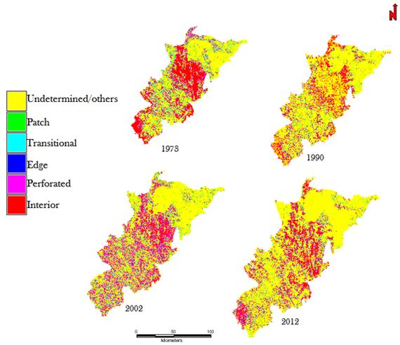
Figure 6: Spatial extent of forest fragmentation in Shimoga division during 1973 to 2012
Table 6: Quantification of forest fragmentation in Shimoga division
| Shimoga division |
| Type of fragments |
1973 |
1990 |
2002 |
2012 |
| Patch |
3.68 |
1.95 |
3.05 |
2.13 |
| Transitional |
6.23 |
8.05 |
6.73 |
4.26 |
| Edge |
1.44 |
1.04 |
1.10 |
1.23 |
| Perforated |
11.89 |
18.00 |
17.06 |
10.49 |
| Interior |
22.90 |
14.20 |
13.83 |
12.91 |
| Undetermined/other category |
53.86 |
56.76 |
58.23 |
68.97 |
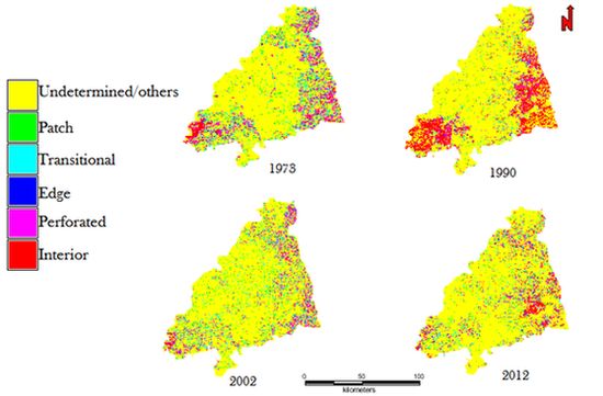
Figure 7: Spatial extent of forest fragmentation in Bhadravathi division
Table 7: Quantification of forest fragments in Bhadravathi division
| Bhadravathi division |
| Type of fragments |
1973 |
1990 |
2002 |
2012 |
| Patch |
5.57 |
4.52 |
4.12 |
3.15 |
| Transitional |
6.62 |
6.82 |
5.03 |
4.42 |
| Edge |
0.90 |
0.93 |
0.58 |
0.91 |
| Perforated |
7.15 |
7.35 |
6.57 |
5.42 |
| Interior |
4.10 |
3.58 |
2.58 |
3.79 |
| Undetermined/other category |
75.66 |
75.74 |
80.12 |
82.31 |
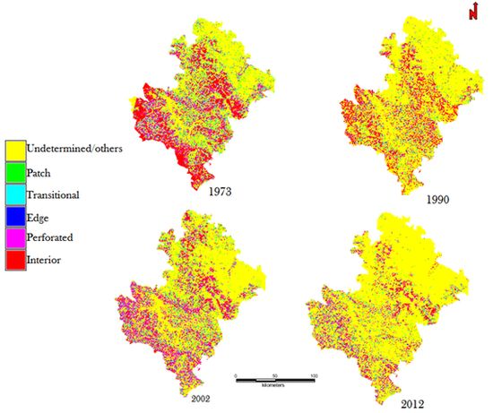
Figure 8: Spatial extent of forest fragmentation in Sagara division
Table 8: Quantification of forest fragments in Sagar division
| Sagar division |
| Type of fragments |
1973 |
1990 |
2001 |
2010 |
| Patch |
3.12 |
2.02 |
3.12 |
1.80 |
| Transitional |
5.82 |
2.96 |
5.82 |
3.34 |
| Edge |
0.93 |
0.92 |
0.93 |
0.87 |
| Perforated |
9.66 |
15.10 |
13.90 |
7.65 |
| Interior |
15.90 |
13.99 |
9.66 |
4.76 |
| Undetermined/other category |
64.57 |
65.01 |
66.57 |
81.58 |
CONCLUSION
Spatio-temporal changes in land cover highlight the decline of vegetation cover from 96.57 (1973) to 91.72 %( 2012). Built-up has increased from 0.63% (1973) to 2.32% (2012) and forest vegetation decreased from 43.83% (1973) to 22.33% (2012). The results highlight conversion of forests to agriculture, industrial and cascaded developmental activities acted as major driving forces of degradation.Forest fragmentation analysis indicated that domination of forests receded during post 90’s with the formation of patch and edge forest in all three divisions. Land use changes from forests to non-forests with intensified human interference had been very high especially in Bhadravathi division. Interior forest decreased by 12% during 4 decades. The extent of interior forests ranges from 12.91 (Shimoga) followed by 4.76 (Sagar) and 3.79 % (Bhadravathi). During the last four decades the interior forest declined from 22.9 (1973) to 13 % (2012) in Shimoga, and 15.90 (1973) to 4.76% (2012) in Sagar, and 4.10 (1973) to 3.79 % (2012) in Bhadravathi divisions emphasizing the need for an immediate eco-restoration measures to arrest fragmentation and consequent reduction in goods and services apart from the increase of human animal conflicts.
REFERENCES
- Bhatta, B., Saraswati, S., and Bandyopadhyay, D. 2010a. Quantifying the degree-of-freedom, degree-of-sprawl, and degree-of-goodness of urban growth from remote sensing data. Applied Geography, 30(1), 96–111.
- Boyle, T.J.B. 2001. Interventions to enhance the conservation of biodiversity. 82-101. In: J. Evans (ed.), The Forest Handbook.Blackwell Science. Oxford, U.K.
- Buiten, H.J, 1988. Matching and mapping of remote sensing images: aspects of methodology and quality. Proceedings 16th ISPRS-Congress, Kyoto, July 1–10, 1988 Vol. 27-B10 III: 321–330.
- Forman, R.T.T. 1995. Some general principles of landscape and regional ecology. Landscape Ecology, 10: 133-142.
- Forman, R.T.T. 1997. Land Mosaics: The Ecology of Landscapes and Regions. Cambridge University Press, New York.
- Griffiths, G.H., Lee J. &Eversham, B.C., 2000. Landscape pattern and species richness, regional scale analysis from remote sensing.International Journal of Remote Sensing, 21: 2685-2704.
- Gustafson, E.J. 1998. Quantifying landscape spatial pattern: what is the state of the art? Ecosystems 1:143-156
- Jensen. J. R. and D.L. Toll, 1982. Detecting residential land use development at the urban fringe, Photogram. Eng. Remote Sensing 48:629–643.
- Jha, C.S., L. Goparaju, A. Tripathi, B. Gharai, A.S. Raghubanshi& J.S. Singh. 2005. Forest fragmentation and its impact on species diversity: an analysis using remote sensing and GIS. Biodiversity and Conservation 14: 1681-1698.
- Jixian Zhang, Yong hong Zhang, 2007. Remote sensing research issues of the National Land Use Change Program of China ISPRS Journal of Photogrammetry and Remote Sensing, 62(6):Pages461-472.
- Laurance, W.F., Laurance S.G. &Delamonica P., 1998. Worldwide forest campaign news: Tropical forest fragmentation and greenhouse gas emissions. Forest Ecology and Management 110: 173-180.
- Nelson R.F, 1983. Detecting forest canopy change due to insect activity using Landsat MSS, Photogram. Eng. Remote Sensing 49:1303–1314.
- O’Neill, R.V., C.T. Hunsaker, K.B. Jones, K.H. Riitters, J.D. Wickham, P.M. Schwartz, I.A. Goodman, B.L. Jackson & W.S. Baillargeon. 1997. Monitoring environmental quality at the landscape scale. Bioscience 47: 513-519.
- Ramachandra T. V., Uttam Kumar, Diwakar P. G. and JoshiN. V., 2009.Land cover Assessment using À Trous Wavelet fusion and K-Nearest Neighbour classification Proceedings of the 25th Annual In-House Symposium on Space Science and Technology, 29 - 30 January 2009, ISRO - IISc Space Technology Cell, Indian Institute of Science, Bangalore.
- Ramachandra T.V and Bharath A.H.,Spatio-Temporal Pattern of Landscape Dynamics in Shimoga, Tier II City, Karnataka State, India, International Journal of Emerging Technology and Advanced Engineering, vol 2(9), pp. 563 – 576, 2012b.
- Ramachandra T.V., Bharath A.H. and Durgappa D.S., Insights to urban dynamics through landscape spatial pattern analysis, Int. J Applied Earth Observation and Geoinformation, vol. 18, pp. 329-343, 2012a.
- Ramachandra. T.V and Uttam Kumar, 2011. Characterisation of Landscape with Forest Fragmentation Dynamics, Journal of Geographic Information System, 3:242-254
- Ramachandra. T.V., Bharath.H.Aithal and Sreekantha S, 2012b. Spatial Metrics based Landscape Structure and Dynamics Assessment for an emerging Indian Megalopolis, International Journal of Advanced Research in Artificial Intelligence, 1(1), 48-57.
- Riitters, K., J. Wickham, R. O'Neill, B. Jones, and E. Smith. 2000. Global-scale patterns of forest fragmentation. Conservation Ecology 4(2):1-28.
- Roy D.P, Lewis P.E. & JusticeC.O., 2002. Burned area mapping using multi-temporal moderate spatial resolution data a bi-directional reflectance model-based expectation approach, Remote Sensing of Environment 83:263–286.
- Saunders, D.A., Arnold, G.W.,Burbridge, A.A. & Hopkins A.J.M., 1987.Nature Conservation, the Role of Remnants of Native Vegetation, Surrey Beatty. Chiiping Norton, Sydney, Australia.
- Trani, M.K. and R.H. Giles, Jr. 1999. An analysis of deforestation: metrics used to describe pattern change. Forest Ecology and Management. 114:459-470.
- Turner, M.G & R.H. Gardner. 1991. Quantitative Methods in Landscape Ecology. Springer-Verlag, New York, USA.
- Vogelmann, J.E. 1995. Assessment of forest fragmentation in southern New England using remote sensing and geographic information system technology. Conservation Biology, 9(2):439-449.
- Wickham, J.D., K.B. Jones, K.H. Riitters, T.G. Wade and R.V. O’Neill. 1999. Transitions in forest fragmentation: implications for restoration opportunities at regional scales. Landscape Ecology14: 137-145.
- Wilkie, D.S, & Finn, J.T, 1996. Remote Sensing Imagery for Natural Resources Monitoring. Columbia University Press, New York. Page 295.
