Results

Image processing algorithm can be considered successful, if it provides good results on images with a wide variety of areas covered. These image processing algorithms are also implemented in a controlled manner under adverse conditions depending upon the input and desired output. This chapter highlights the results obtained from implementation of the algorithms (discussed in chapter 3 and chapter 4) on LISS-3 MSS and MODIS data.

The chapter is arranged in 5 sections. The first and second section (5.1 and 5.2) discusses the Land cover analysis using NDVI (Normalised Difference Vegetation Index) from LISS-3 MSS and MODIS bands respectively. The third section (5.3) deals with the LISS-3 image processing. The fourth section (5.4) is divided into 3 sub-sections. The first subsection (5.4.1) shows the result obtained from MODIS Bands 1 to 7 classification using Maximum Likelihood Classifier, Spectral Angle Mapper, Neural Network and Decision Tree Approach. The second subsection (5.4.2) shows the results of the implementation of above algorithms on Principal Components (PC) of MOIDS bands 1 to 36. Results of the above algorithms on Minimum Noise Fraction (MNF) Components of MODIS bands 1 to 36 is shown in sub section 3 (5.4.3). The last section (5.5) of this chapter deals with the results obtained from linear spectral unmixing of MODIS imagery.

The LISS-3 MSS data (of spatial resolution 23.5 m) were used as a high resolution data for land cover mapping.

The LISS-3 images (having bands in Green, Red and Near-infrared wavelengths) were geometrically corrected by using ground control points (GCPs) and reference toposheets of the Survey of India. These GCPs were collected in the field using hand held GPS. The images were resampled using nearest neighbourhood technique with an overall RMS error of 0.11.

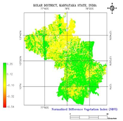
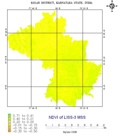
NDVI was generated using LISS-3 data for land cover analysis, is given in figure 5.1 ranges from 0.71 to -0.50. NDVI gave land cover (vegetation/green versus non-vegetation/non-green) information. The NDVI showed that 46.03% of the area has vegetation (agriculture, forest and plantations /orchards) and the remaining 53.98 % has non-vegetation (built up land, waste / barren rock / stony and waterbodies).

Figure 5. 1 : NDVI of LISS-3 MSS based on bands 3 (Red) and 4 (NIR).

Figure 5. 2 : NDVI generated using MODIS bands 1 and 2.

As mentioned earlier, MODIS data having coarse spatial resolution (250m) were used for land cover mapping. The acquisition and preprocessing of the MODIS data is discussed in detail in chapter 1 and 2.

Although the original expected geolocation accuracy of the satellite was of 150 m, but nowadays, after several updates which involved the use of parametric and non parametric (GCP's, DEM) methods to eliminate bias and other sources of error, the accuracy of higher level products is of 50 m [131] and according to MODIS web sources it could even be around 40 m [132]. Still, in order to achieve pixel level accuracy, georeferencing was done with the metadata accompanying the original image, GCPs collected in the field using hand held GPS and reference maps (topographic maps of the Survey of India, etc.) with an accuracy of 11 m.

The spatial resolution of MODIS (MOD 09 Surface Reflectance 8-day L3 global Products) bands 1 and 2 are 250 m, while bands 3 to 7 have pixel sizes of 500 m. Bands 3-7 were resampled by nearest neighbourhood technique to 250 m for easy processing, overlaying and comparison, and for analysis consistency. The first 2 bands of the MODIS were stacked with the remaining 5 bands (bands 3 to 7). Finally, the first seven bands with spatial resolution of 250 m were used for further processing.

The MODIS L1B product (MOD 02 Level-1B Calibrated Geolocation Data Set) with 36 spectral bands has a spatial resolution of 1 km. These bands were resampled to 250 m, as getting a pure pixel of 250 x 250 m was relatively easier compared to still coarser resolutions. All these bands were reprojected from Sinusoidal projection to Polyconic projection with Evrst 1956 as the datum, followed by masking of the study area.

5.2.2 Land Cover Analysis

Red and near-infrared bands of the MODIS sensor at 250 m spatial resolution were used to compute NDVI, which is given in figure 5.2. NDVI ranges from 0.35 to -0.54, indicating that 47.35% of the area under vegetation (agriculture, forest and plantations / orchards) and the remaining 52.65 % under non-vegetation (built up land, waste / barren rock / stony and waterbodies).

The classifiers work at the pixel level with spectrally distinctive classes. If this condition is not met, there is risk of confusion between the classes, leading to poor classification accuracies. This issue is particularly important when working with few spectral bands as the ability to identify a specific class diminishes with fewer bands, and subsequently less information is depicted.

The class spectral characteristics for the six land use classes for LISS-3 MSS bands 2 (Green), 3 (Red) and 4 (NIR) were determined and the Transformed Divergence matrix (table 5.1) helped in distinguishing different classess. The values in the table range from 0 to 2.0. Values greater than 1.9 indicate that the ROI pairs have a very good separability. It is seen that the overall separability is good except for agriculture, forest and plantation classes.

Ground truth obtained from field and other ancillary data were used for the LISS-3 MSS classification. This was done in two steps: unsupervised classification and supervised classification.

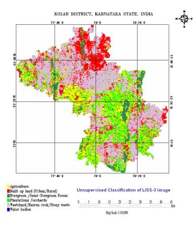
Histograms were generated to ascertain the number of likely land cover categories based on the number of distinguishable peaks. Unsupervised classification was performed on this data using the K-means clustering algorithm. The results of the unsupervised classification (given in figure 5.3), indicated that the mapping of the classes can be done accurately with the MLC classifier, giving an overall good representation of what was observed in the field.

Figure 5. 3 : Unsupervised classification of LISS-3 image.

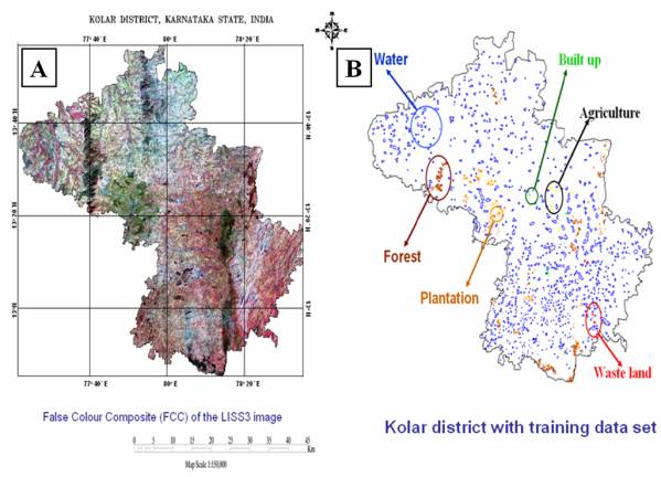
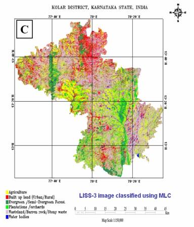
Figure 5. 4 : (A) False Colour Composite of the LISS-3 image, (B) Kolar district with training data set, (C) Supervised Classified image of LISS-3 MSS.

False colour composite (FCC) was generated from the LISS-3 MSS data after geometric correction by assigning blue to green, green to red and red to near-infrared bands respectively and is given in figure 5.4 (A). The heterogeneous patches (training polygons) were chosen for the field data collection is given in figure 5.4 (B). Supervised classification using GMLC was performed with the ground truth data. Care was taken to see that these training sets are uniformly distributed representing / covering the study area. The supervised classified image shown in figure 5.4 (C) was validated by field visit and by overlaying the training sets used for classification (Accuracy Assessment, discussed in chapter 6).

The percentage statistics of each class in unsupervised and supervised classification are listed in table 5.2.

5.4 Classification of MODIS data

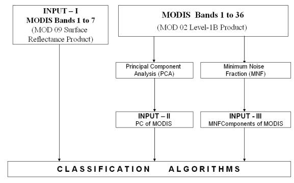
Three different types of input were given to the various hard classification algorithms as shown in figure 5.5.

•  MODIS Bands 1 to 7 ( MOD 09 Surface Reflectance 8-day L3 global Products)

•  Principal Components of MODIS Bands 1 to 36 (MOD 02 Level-1B Calibrated Geolocation Data Set)

•  MNF Components of MODIS Bands 1 to 36 (MOD 02 Level-1B Calibrated Geolocation Data Set)

Figure 5. 5 : Different MODIS inputs to the hard classification algorithms.

The MODIS bands 1 to 7 (MOD 09 Surface Reflectance 8-day L3 global Products) were used as the “first input” to various classification algorithms. The MODIS Surface-Reflectance bands (MOD 09) is computed from the MODIS Level 1B land-bands 1 to 7, (explained in chapter 1), which is an estimate of the surface spectral reflectance for each band comparable to measurements at ground level in absence of atmospheric disturbances (scattering or absorption). The class spectral characteristics for the six classes defined in this study across the first seven bands of the MODIS sensor were determined and the Transformed Divergence matrix given in table 5.3, shows a similar pattern that helped in determining the separability among the various classes. It is seen that the overall separability is generally good compared to LISS3 (table 5.1).

Unsupervised Classification

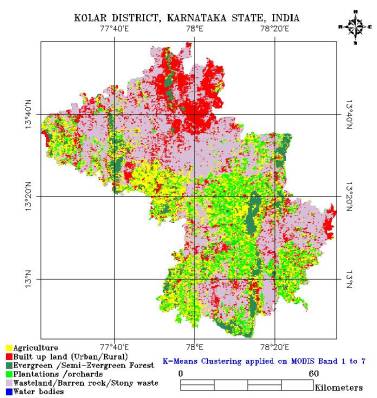
Unsupervised classification of the MODIS 7 bands was performed using K-means algorithms. Initial clustering of the bands into 25 classes was attempted at various thresholds. The maximum number of pixels was classified when the threshold was maintained at 0.8. Later on, the classes were merged and finally, the unsupervised classification resulted in 6 land cover classes as shown in figure 5.6. A histogram generated for FCC show 6 peaks, indicating 6 categories of land uses. The statistics for the various classes are shown in table 5.4.

Figure 5. 6 : Unsupervised Classification on MODIS Bands 1 to 7.

Supervised Classification

Supervised classification on MODIS bands 1 to 7 was performed using Gaussian Maximum Likelihood Classifier (GMLC), Spectral Angle Mapper (SAM), Neural Network (NN) and Decision tree Approach (DTA).

•  A FCC was created using MODIS bands 1 (Red), 2 (NIR) and 4 (Green). The heterogeneous patches were identified for training data collection. The MODIS bands 1 to 7 were classified by GMLC technique. At a threshold of 0.001, the 7 bands gave a good representation of the land cover classes.

•  The above bands were then classified using the SAM technique. At an angle of 0.5 radians, the output of the classified map also represented the 6 land cover classes.

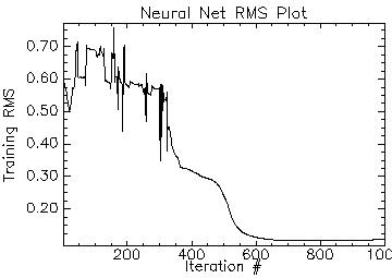
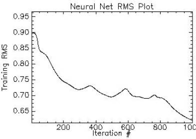
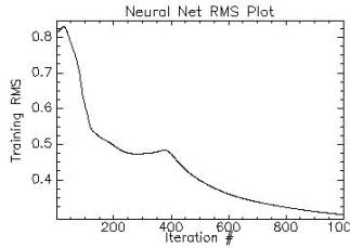
• NN was used for classifying MODIS data of 7 bands. The process of training the neurons was time consuming. Although NN is considered to be one of the most robust techniques for classification of remotely sensed data, yet, controlling the training process in NN was difficult. Figure 5.7 shows neural network RMS plot. The training process of the neurons was iterated 1000 times to see the converging point. The iterations stopped with the overall RMS 0.09. The number of hidden layer was kept at 1 and the output activation function was kept 0.001. The output activation function was increased in steps to see the variations in the classification. The training momentum was initially 0 and was increased gradually. The training RMS exit criteria were 0.1, the training threshold contribution was kept 0.1, and the training rate was maintained 0.2 during the training process.

Figure 5. 7 : Plot of training RMS vs. iterations of NN applied on MODIS bands 1 to 7.

• Decision Tree approach with See5 was used by the knowledge classifier to classify the MODIS 7 bands. Thus, this rule based approach was a more controlled kind of classification process among all the other techniques. Table 5.4 shows the total number of rules generated by the decision tree classifier, the maximum and the minimum confidence level for each class to control its accuracy. The confidence level shows a feasible way of rules by probability forms, and it also raises a flexibility of data error tolerance. The table also highlights the number of rules used for classification at a confidence level of 0.6. The procedure is described below:

•  A set of points were defined as training sites based on a priori knowledge of the study area, for various land cover classes in the data set.

•  The scaled reflectance values for land cover classes were extracted for the training data.

•  The data were converted into SEE5 compatible format and submitted for extraction of rules.

•  Since the boosting option changes the exact confidence of the rule, the rules were extracted without boosting option. A 10% cut off was allowed for pruning the wrong observations.

•  Once the rules were framed by the SEE5, these rules were ported into Knowledge engineer to make a knowledge based classification schema. It was ensured that 90% confidence level is maintained for all the classes defined.

•  Subsequently the decision tree schema was applied over the data set to produce the colour coded land cover output.

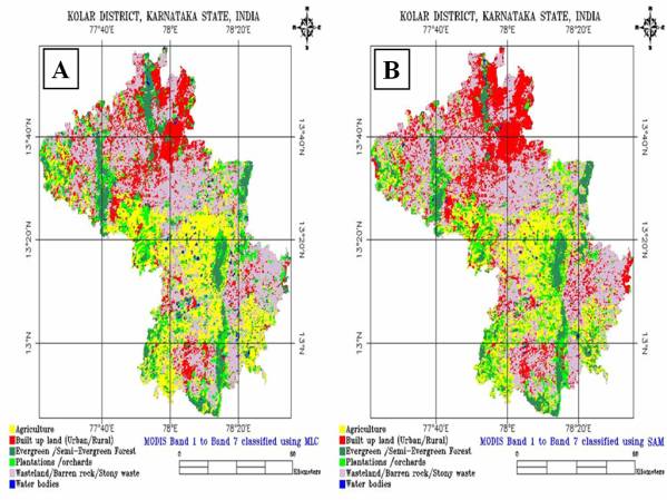
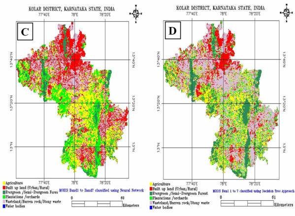
The results obtained from the various classification techniques for MODIS bands 1 to 7 are listed in table 5.5 for comparative analysis. From the table it is clear that in the neural network based classification there is an increase in the built up land and plantation classes with a decrease in the waste land percentage. The percentage of vegetation (agriculture, forest and plantation) in K-means clustering was 40.77%, 44.34% (in MLC), 38.06 (in SAM), 49.15% (in NN) and 44.61% (in Decision Tree). The percentage of non-vegetation (built up, waste land/ Barren rock / Stony waste and waterbodies) were found to be 59.23% in K-means clustering, 55.64% (in MLC), 61.95% (in SAM), 51.13% (in NN) and 55.39% (in Decision Tree) approach respectively. Figure 5.8 shows the corresponding classified images.

Figure 5. 8 : Supervised Classification using (A) MLC, (B) SAM, (C) NN and (D) Decision Tree Approach on MODIS Bands 1 to 7.

Principal Component Analysis (PCA) was performed on MODIS 36 bands (MOD 02 Level-1B Calibrated Geolocation Data Set) of spatial resolution 250m. The covariance matrix and the correlation matrix were calculated and eigenvalues are listed in table 5.6.

It is observed, that only the first few bands have higher information. The first five bands of the PCA were chosen for further analysis based on higher eigenvalues, and the information content that was perceived from visual interpretation of the images through false colour composite. These 5 components were used as the “second input” to the classification algorithms.

Transformed Divergence matrix is given in table 5.7 indicated that except built up all other classes are well separable across PC's.

•  PC's were first classified by GMLC technique and at a threshold of 0.001, gave the best representation of the land cover classes.

•  PC's were then classified using the Spectral Angle Mapper technique. Here the spectral angle was set different for each class (5 for agriculture, 5 for built up, 0.05 for forest, 0.02 for plantation, 3 for forest and 0.02 for waterbodies) after iterations of tuning the angle between the class spectra and the reference spectra to avoid misclassifications.

Neural Network technique was applied to PC's. After several iterations of the training process, stability was achieved. Figure 5.9 shows the NN plot of the training process iteration versus the RMS error obtained. The training curve obtained here was very smooth and the process of training the neurons converged at 1000 iterations. The number of hidden layers was kept at 1 and the output activation function was maintained at 0.001. It was seen that as the number of hidden layer is increased, the training process takes more time, giving irrelevant outputs. So, maintaining the hidden layer at 1 was justified with this result. The training momentum was initially kept 0 and was later on increased in small steps when it was observed that the training of neurons is reaching stability.

Figure 5. 9 : Plot of training RMS vs. iterations of NN applied on PCA bands (MODIS Bands 1 to 36).

•  Decision Tree approach using See5 and the knowledge engineer was used to classify PC's. For each training site, a level of confidence in characterisation of the site was recorded. Table 5.8 shows the total number of rules generated, the maximum and the minimum confidence level for each class and the number of rules used for classification at a confidence level of 0.92. Here the image was classified into 16 classes initially and were ultimately merged into six categories.

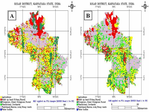
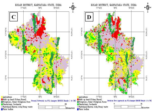
The results obtained from these classification techniques are listed in table 5.9. The percentage of vegetation (agriculture, forest and plantation) was 45.56% (in MLC), 43.67 (in SAM), 45.98% (in NN) and 43.12% (in Decision Tree). The percentage of non-vegetation (built up, waste land / barren rock / stony waste and waterbodies) were found to be 54.41% (in MLC), 56.31% (in SAM), 54.00% (in NN) and 56.88% (in Decision Tree) approach respectively. Figure 5.10 shows the classified images using MLC, SAM, NN and DTA.

Figure 5. 10 : Supervised Classification using (A) MLC, (B) SAM, (C) NN and (D) Decision Tree Approach on PC's.

Minimum Noise Fraction (MNF) was performed on the MODIS bands 1 to 36. The covariance matrix, correlation matrix, eigenvectors and eigenvalues were computed for the MNF and the eigenvalues are listed in table 5.10.

The first five components of MNF were chosen depending on their higher eigenvalues for classification. The output of MNF reflected more information content, yet the image obtained were more pixilated and appeared to be arranged in a brick line fashion in some places on the image. To avoid noise, the other components of MNF were ignored as they that had lower signal-to-noise ratio. These 5 components were used as the “third input” to the various classification algorithms. The Transformed Divergence matrix is given in table 5.11, showed that the overall inter class separability is very high due to reduced noise.

•  The pixels in the MNF components were not very distinct and were clustered into mini groups (comprising of two or three pixels). Though, the class separability was very good, yet it was difficult to classify each pixel based on signature, since the image was slightly pixilated. The MNF components were classified by GMLC technique at a threshold of 0.001.

•  MNF components were then classified using the SAM technique. At an angle of 5 radians, all the classes represented the land cover classes well (except water, which was classified at an angle of 0.2 radians).

•  NN was used to classify the MNF components. The graph in figure 5.11 was relatively smooth for the whole process and shows the training process converging at 1000 iterations. The hidden layer was 1 and the output activation function was 0.001. The training momentum was initially 0 and was increased gradually. Other observations were similar to that of PCA classification. The RMS error at the completion of the process was 0.29.

Figure 5. 11 : Plot of training RMS vs. iterations of NN applied on MNF Components.

•  Decision Tree approach was used to generate the rules for the knowledge classifier to classify the image. The threshold factor was maintained at 0.7. Table 5.12 shows the total number of rules generated, the maximum and the minimum confidence level for each class and the number of rules used for classification at a confidence level 0.7.

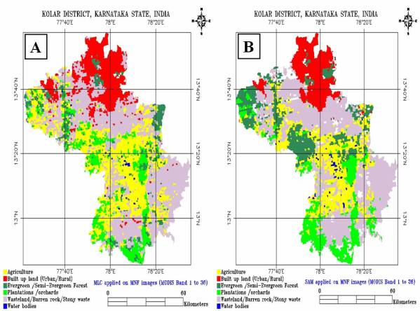
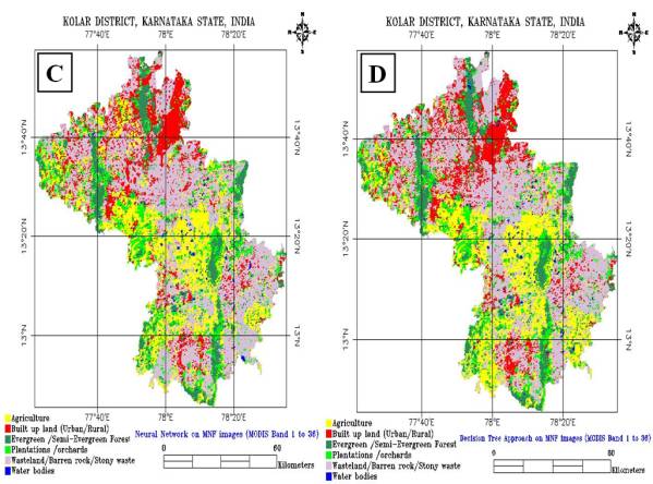
The results obtained from these classification techniques are listed in table 5.13. In SAM classification there is an increase in the forest and plantation class whereas in ML classification, agriculture is high and on the other hand forest and waterbodies show a relatively low contribution to the land cover class percentage. In the decision tree approach, there is a slight decrease in the water class percentage. Vegetation (agriculture, forest and plantation) contributes 45.37% (in MLC), 46.90% (in SAM), 39.81% (in NN) and 46.29% (in Decision Tree) and non-vegetation (built up, waste land/ Barren rock / Stony waste and waterbodies) contributes 54.96% (in MLC), 53.08% (in SAM), 60.46% (in NN) and 53.71% (in Decision Tree) approach, respectively. The classified images obtained are shown in figure 5.12

Figure 5. 12 : Supervised Classification using (A) MLC, (B) SAM, (C) NN and (D) Decision Tree Approach on MNF components.

The overall representation of various classes with respect to different classification algorithms compared on the basis of percentage area is depicted in Table 5.14. The table shows the uniform distribution of agriculture, forest, plantation and waterbodies classes whereas built up has increased and waste land fell below average line in NN based classification for MODIS Bands 1 to 7.

Table 5. 14 : Land cover classes compared on the basis of different algorithms versus percentage area.

The hard classification techniques discussed above classified each pixel to a known single land cover class. Pixels with coarse spatial resolution are likely to have more than one land cover type posing the problem of mixed pixels. Hence linear unmixing was attempted through soft classification of MODIS data. LSU generated a series of abundance maps, one for each class considered, instead of a single one depicting all classes present in an image. Here, every pixel was not assigned exclusively to one class, but was part of many, modeled by a linear model.

MNF transformation was performed on the seven bands of the MODIS (MOD 09 Surface Reflectance 8-day L3 global Products). It was used to determine the inherent dimensionality of the data, to reduce noise and computational requirements for subsequent processing. By using only the coherent portions in subsequent processing, the noise is separated from the data, thus improving spectral processing results.

5.5.2 Endmember collection

The endmembers were extracted directly from the data without using existing spectral libraries. The selections of endmembers to train the algorithm were done in several steps.

The MNF bands were used in the PPI (as explained in chapter 4), processing designed to locate the most spectrally pure pixels typically corresponding to mixing endmembers. A PPI image was created in which the digital number of each pixel corresponded to the number of times that pixel was recorded as extreme. A histogram of these images showed the distribution of hits by the PPI. A threshold was interactively selected using the histogram and used to extract only the purest pixels in order to keep the number of pixels to be analyzed to be minimum. These pixels were used as input to an interactive visualization procedure for separation of specific endmembers.

Scatter plots of the bands also helped in locating some of the purest endmembers by taking the extreme corner pixels. In two dimensions, if only two endmembers mix, then the mixed pixels fall in a line in the histogram. The pure endmembers fall at the two ends of the mixing line. If three endmembers mix, then the mixed pixels fall inside a triangle, four endmembers fall inside a tetrahedron, etc. Mixtures of endmembers fill in between the endmembers. All mixed spectra are interior to the pure endmembers, inside the simplex formed by the endmember vertices, because all the abundances are positive and sum to unity. These set of mixed pixels were used to determine how many endmembers were present and helped in estimating their spectra.

The spectra are the points in an n-dimensional scatter plot, where n is the number of bands. The coordinates of the points in n-space consist of ‘n' values that are simply the spectral reflectance values in each band for a given pixel. The distribution of these points in n-space was used to estimate the number of spectral endmembers and their pure spectral signatures, and provided an intuitive mean to understand the spectral characteristics of materials.

The pixels from the spectral bands were loaded into an n-dimensional scatter plot and rotated on the visualisation tool until points or extremities on the scatter plot were exposed. These projections were marked using region of interest (ROI) tool and then were repeatedly rotated in lesser dimensions to determine if their signatures were unique. Once a set of unique pixels were defined, then each separate projection on the scatter plot (corresponding to pure end member) was exported to a ROI in the image. Mean spectra were then extracted for each ROI to act as endmembers for spectral unmixing. These endmembers were then used for subsequent classification and other processing.

A few of the training sets were exclusively collected in the field, corresponding to pure pixels. These training data were overlaid on the FCC of the image and a region of interest (ROI) was created, thus enabling direct selection of assumed pure pixels from the images. This was done for all classes (agriculture, built up, forest, plantation, waste land and waterbodies) where a clear distinction between their pixels was possible.

Finally, these ROIs obtained by different methods were merged into six classes and exported as endmembers.

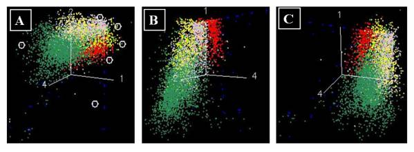
The spectral characteristics of the endmembers were analysed by plotting the endmembers and obtaining the Transformed Divergence matrix which showed a clear separability between the endmembers. These endmembers were then rotated using the n-dimensional visualiser. Snapshots of the visualisation are shown in figure 5.13. The endmembers are marked using a white circle in figure

5.13 (A). It shows that the endmembers selected for the analysis are well separable and can be distinguished from each other.

Figure 5. 13 : 3-Dimensional visualisation of the Endmembers showing their separability.

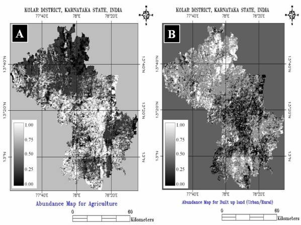
Linear Unmixing was performed using the endmember obtained, and keeping the unit sum constraint as 1. Fraction images corresponding to each endmember were generated. The visual inspection of the fraction images shown in figure 5.14 and figure 5.15 indicates that the LSU algorithm was generally capable to detect the patterns present in the supervised classification, but at the same time incurred in significant errors. The proportions of the endmembers in the fraction image ranges from 0 to 1. 0 indicates absence of the endmember and increasing value shows higher abundance with 1 representing 100% presence of the endmember in a particular pixel.

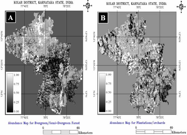
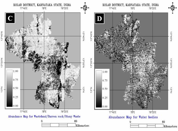
This is evident when looking at the fraction map for Agriculture (figure 5.14 (A)) which has mixed at several places with forest / plantations . The first exhibits an over detection along a wide range of the central portion of the area. Plantation and agriculture seems to have mixed at a few places when compared to the hard classified image. The overall representation of wasteland / barren rock / stone was better and in the case of waterbodies, there is a clear case of false detection of the endmember in the northern region of the district and, particularly in the central portion of the district. By and large, other classes show a better behaviour, with distribution and relative values more closely resembling the outputs of the supervised classification, though still some errors exist.

Figure 5. 14 : (A) Gray scale Abundance Maps for Agriculture and (B) Built up land (Urban / Rural ).

Figure 5. 15 : Gray scale Abundance Maps for Evergreen / Semi-Evergreen Forest (A) Plantations/orchards (B) Wasteland/Barren rock/Stone (C) and Waterbodies (D). Bright pixels represent higher abundance of 50% or more stretched from black to white.

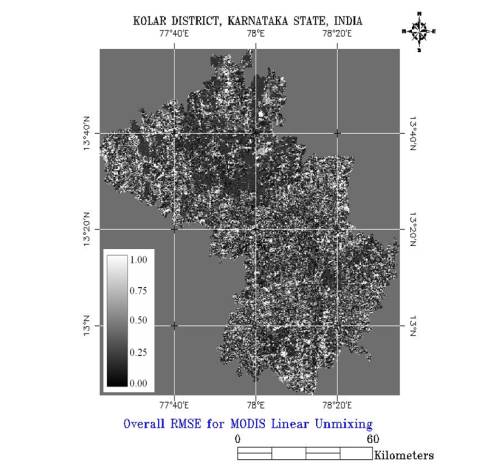
It has to be noted that output values of the different MPF's (Material Pixel Fractions) many times fell beyond acceptable limits, showing highly positive and negative values, usually corresponding to areas of high RMSE (figure 5.16). In those cases, values that exceeded 1 were considered to be 1 and values under 0 were assimilated to this cipher. In figure 5.16, 0 (black) represents no error and 1 (white) represents high error in the fraction image.

Figure 5. 16 : Overall RMSE for MODIS. Bright pixels represent high error.

Overall, the MPF images show good correspondence between the visual patterns and relative values of the fractions when compared with the hard supervised classification suggesting a better behaviour in the distribution of the endmembers. There are many areas where proportions of agriculture are properly predicted, mainly in the western central portion of the study area however, there is clear underestimation in the south central region of the district. Errors can be seen in the wrong detection of waterbodies showing high discrepancies.

As the experimental results show, classes identified in remote-sensing data may exhibit an interclass variability too high to allow the unique linear spectral unmixing of single pixels. Parametric representation of the constituent pure classes used for linear unmixing does not properly represent local classes since the sampling error may be significant and, in most cases, parametric probability density functions are valid when certain assumptions are met that do not always hold in practice [133]. The variability of the pixels that represent the local pure classes then is responsible for the uncertainity with which the mixture proportions can be identified.