Soft Classification: Spectral Unmixing

Low spatial resolution space borne sensors (such as MODIS) improve the ability to image large areas of earth's surface quickly and inexpensively. The emergence of hyperspectral technology based on the spectral imaging principle has removed the limitation of few spectral bands as is the case with multispectral data. Spectral imaging is the mapping of each spatial resolution element the pixel , to a quantized energy spectrum. A variety of factors interact to produce the signal received by the imaging spectrometer for any pixel. Spatial mixing of materials within a pixel footprint result in spectrally mixed reflected signals. Classification of these pixels is necessary for identifying and discriminating the different spatial features present on the earth's surface.

One of the most popular methods used for classifying remotely sensed data is to identify the pixels containing user-specified categories. This image classification routine assumes “pure” or homogeneous pixels and allocates a pixel to the maximally “similar” class, which is then expected to be the class of maximum occupancy within the pixel [111]. A variety of other classification methods, such as spectral matched filter [112], mixture tune matched filtering and spectral angle mapper [113] are appropriate when pixels do not contain mixtures of materials with correlated spectra, have been developed.

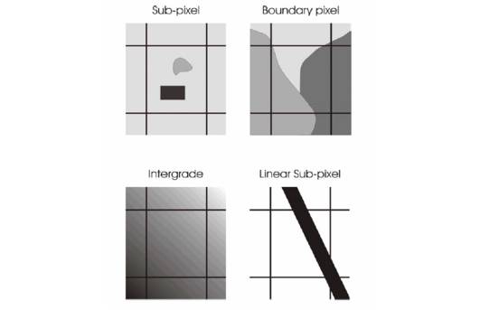
Natural surfaces are rarely composed of a single uniform category. For example, each pixel produced by MODIS covers approximately 62,500 m²– 1,000,000 m² on the ground (for pixel sizes of 250 m and 1 km, respectively) and is thus typically larger than the surface expression of features on the earth's surface. Therefore, it is seldom the case that one is interested in classifying a single pixel, unless of course the application is specifically oriented toward identifying objects of subpixel size [111]. On the other hand, it is often the case in remote sensing that one wants to deal with identification, detection and quantification of fractions of the target materials for each pixel for diverse coverages in a region. Thus the problem of mixed pixel classification is a major issue in remote sensing and geography and many approaches have been developed to deal with it. For those cases, a more suitable way of extracting information is to estimate the composition of each pixel by spectral unmixing . This approach is known as soft classification . Subpixel classifiers deal with the mixed pixel problem. Mixed pixels are normally found in boundaries between two or more mapping units, along gradients, etc. when the occurrence of any linear or small subpixel object takes place as shown in figure 4.1.

Figure 4. 1 : Four cases of mixed pixels [116].

To resolve the mixed pixel problem, the scale and linearity of the mixture have been investigated by several researchers, (e.g. [115], [116], [21], [111] and [117]). There have been two different models. The microscopic mixture model considers mixing as nonlinear. It deals with not only with the pixel of interest, but also neighbouring pixels. The macro spectral mixture model assumes no interaction between materials and a pixel is treated as a linear combination of signatures resident in the pixel with relative concentrations. This is also referred as Linear Mixture Model (LMM). The basic idea of the LMM is the assumption of insignificant multiple scattering between the different class types, i.e., each photon that reaches the sensor has interacted with just one class type. Therefore, the received energy can be considered as a sum of the energies received from each class, which depends on the characteristics of the class type and the area covered by that type.

4.2 Linear Unmixing

To address the problem of mixed pixels, there is a growing interest in the use of techniques designed to estimate class proportions (rather than a single class label) for individual pixels (eg. [118], [119]). Such methods attempt to model the spectral response from a mixture of classes and the approach is generically termed as ‘mixture modelling'. If the mixture model can provide information from MODIS data compared to that normally obtained from higher resolution data, albeit at 250 m to 1 Km resolution, then MODIS data is particularly attractive for many applications because of their relatively low cost, larger ground coverage and higher temporal resolution than many other systems [22].

The linear unmixing method [120], is used for solving the mixed pixel problem of MODIS data. The hypothesis underlying linear unmixing is that the spectral radiance measured by the sensor consists of the radiances reflected by all of these materials, summed in proportion to the sub-pixel area covered by each material. To the degree that, this hypothesis is valid, and that the ‘endmembers' are given by the reference spectra of each of the individual pure materials, and under the condition that these spectra are linearly independent, then in theory one can deduce the makeup of the target pixel by calculating the particular combination of the endmember spectra required to synthesize the target pixel spectrum. In dealing with coarse resolution data, it is assumed that the spectral response due to ground class mixtures varies linearly with the relative proportions of those classes. Sites of ‘pure' land cover for each class (or ‘component') of interest are identified, and their spectra used to define ‘endmember' signatures. These signatures lie at extreme ends of a continuum in spectral feature space. According to this linear mixture model, the position of the spectral signature of an input pixel along this continuum indicates directly the percentage cover for each component [21].

A linear relation is used to represent the spectral mixture of targets within the pixel of remote sensing system. Based on this assumption, the response of each resolution element (pixel) of the remote sensing system in any spectral wavelength can be considered as a linear combination of the responses of each component, which are assumed to be in the mixture. Thus, each image pixel, which can assume any value within the gray scale, contains information about the proportion and spectral response of each component within the ground resolution unit.

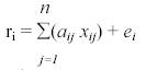
Hence, given a hyperspectral image, it is possible to model each pixel spectrum of this image as a linear combination of a finite set of components:

r₁ = a₁₁ * x₁ + a₁₂ * x₂ + ... + a_1n * x_n + e₁
r₂ = a₂₁ * x₁ + a₂₂ * x₂ + ... + a_2n * x_n + e₂
r_m = a_m1 * x₁ + a_m2 *x₂ + ... + a_mn * x_n + e_m

or

where,

r_i = Spectral reflectance of the pixel in ith spectral band of a pixel containing one or more components.

a_ij = Spectral reflectance of the jth component in the pixel for ith spectral band.

x_j = Proportion value of the jth component in the pixel.

e_j = Error term for the ith spectral band.

The error term (e_i ) is due to the assumption made that the response of each pixel in any spectral wavelength is a linear combination of the proportional responses of each component

j = 1, 2, 3 ... n (Number of components assumed)

i = 1, 2, 3 ... m (Number of Spectral bands for the sensor system)

A linear constraint is added, since the sum of the proportions for any pixel must be one. Also, the proportion values must be non-negative. Considering that in case of the hyperspectral image analysis, the number of components (n) is less than the number of spectral bands (m) of sensor, the system of the equation is over-determined and can be solved by a number of techniques such as the Constrained Least-Squares method [120]. The diagonal elements in equation (4.1) are the pure pixels.

Constrained Least Squares Method (CLSM) estimates the proportion of each component within a pixel by minimizing the sum of squares of the errors [120]. The proportion values must be non-negative, and they also must add to one. In order to solve this problem, a quasi-closed solution method (e.g., a method which achieves the solution by making approximations to the variables in order to satisfy the constraints) is used. For a mathematical derivation of CLSM, please see Annexure C.

The reflected spectrum of a pure feature is called a reference or endmember spectrum. Endmember spectra are extracted under idealized laboratory conditions where reflected spectrum is obtained with a spectrometer focused on a single feature. When this is impractical, the endmembers are derived from imagery manually.

One possible source for the endmember spectra are libraries of spectral reflectance. The risk in using such library spectra is that the library spectra are rarely, if ever, acquired under the same conditions as the air-borne/space-born data. A better match will be obtained if the endmember spectra are taken from the image cube under analysis.

Techniques have been developed to automatically extract endmember spectra from the remotely sensed data set [121]. All these algorithms have been successfully used to determine end-members and unmix several hyperspectral data sets without the use of any priori knowledge of the constituent spectra [122].

Endmember variability was incorporated into mixture analysis by representing each endmember by a set or bundle of spectra, each of which could reasonably be the reflectance of an instance of the endmember. Endmember bundles were constructed from the data itself by a small extension to the method of manually deriving endmembers from the remote sensing data. When applied to remotely sensed images, bundle unmixing produced maximum and minimum fraction images bounding the correct cover fractions and specifying error due to endmember variability. This paper discussed a method by which the endmember bundles and bounding fraction images were created for an airborne visible/infrared imaging spectrometer (AVIRIS) subscene simulated with a canopy radiative transfer/geometric-optical model. Variation in endmember reflectance was achieved using ranges of parameter values including leaf area index (LAI) and tissue optical properties observed in a North Texas Savana. The subscene's spatial pattern was based on a 1992 Landsat Thematic Mapper image of the study region. Bounding fraction images bracketed the cover fractions of the simulated data for 98% of the pixels for soil, 97% for senescent grass, and 93% for trees. Averages of bounding images estimated fractional coverage used in the simulation with an average error of = 0.05 , a significant improvement over other methods with important implications for regional-scale research on vegetation extent and dynamics [123] .

In a study conducted by [124], the endmember spectra have been allowed to have random fluctuations, giving rise to a covariance matrix for the residual that depends on the underlying proportions using linear model. It was shown that under a simple set of models for the variability for both endmembers and abundance, the covariance matrix for the residual is a weighted sum. Generally, the balance is determined by the length scale for changes in the reflectance of any given cover type, and the length scale for changes in surface cover itself; one or other of the two limit models (linear or non-linear) is preferred when these lengths are very different. The attempt could derive an improved representation of the error term, or residual, in the linear mixture model, taking account of the variability of endmember spectra, and of subpixel variation in fractional abundance of surface cover. A few of the endmember extraction techniques used in this study are discussed briefly here.

A dimensionality reduction is first performed using the MNF transformation (refer section 2.3.2 in chapter 2). The next step is the calculation of the pixel purity index for each point in the image cube. This is accomplished by randomly generating lines in the N-dimensional space comprising a scatter plot of the MNF transformed data. All of the points in the space are then projected onto the line. Those pixels that fall at the extremes of the lines are counted. After many repeated projections to different lines, those pixels with a count above a certain threshold are declared “pure”. As a result, there will be many redundant spectra in the pure pixel list. The actual end-member spectra are selected by a combination of intelligent review of the spectra themselves and through N-dimensional visualization [122].

Figure 4. 2 : Scatter plots between two bands typically show a triangular shape, with the data radiating away from the shade-point and A, B, C as the endmembers.

Each scene spectrum maps to a point in this PC space, and the set of all scene spectra constitutes a scatter plot. The endmember spectra occur at the extremities of this scatter plot. The methods most often used to acquire the endmember spectra from the data rely upon computer visualization tools which allow manipulation of this scatter plot, permitting one to project the plot onto an arbitrary plane in the PC or MNF transformed space. This permits an operator to locate the extremities, the endmember spectra, in the scatter plot. The spectra of all the pixels selected from the extremities in this scatter plot then constitute the set of endmember spectra [122].

A study was conducted at Lake Baikal region in Russia by using remote sensing technique and phenological pattern of plants for land cover mapping ( Shimazaki et al ., 2001 ) [2]. A new linear mixture method, a spectral and temporal linear mixing model was proposed, which is developed from both spectral and temporal aspects. To estimate the proportion of components in the mixed pixel, the Linear Mixture Model (LMM) was applied to five temporal scenes of LANDSAT 7/ETM satellite data. The LMM proposed has two steps. In the first step as spectral LMM, the area proportions of each endmember (basic land cover class) for all five scenes were estimated. In the second step as temporal LMM, the annual fluctuations of proportions of each endmember were used as new endmembers. Finally, the proportions of several plants in the mixed pixel were estimated, which had a distinctive phenological pattern. In the proposed model, the characteristics of annual fluctuations of each endmember were used to determine land cover classes. The paper also introduced the method of proposed LMM, though the validation of this LMM was left for the further research.

A model based mixture supervised classification approach in hyperspectral data analysis (Dundar et al ., 2002) [125] favoured the mixture classifier over the simple quadratic classifier. The majority of the cases showed that characterising class densities by a mixture density is useful in obtaining a more precise class definition. However, as with most classifiers, the success of the mixture classifier is also limited by the size of the training data set available. The main difference between a simple quadratic classifier and a mixture classifier is that the former does not guarantee a better performance when a larger training dataset is used during the design process, but the latter usually does, given enough components and separability among classes. The larger the number the training dataset, the more accurately the densities are estimated and hence the better the performance of the mixture classifier.

A successful geologic case analysis of hyperspectral data using an end-to-end approach on Airborne Visible/Infrared Imaging Spectrometer (AVIRIS) data was attempted by ( Kruse et al ., 1997 ) [58]. It included data calibration to reflectance, use of linear transformation to minimize noise and determine data dimensionality, location of the most spectrally pure pixels, extraction of endmember spectra, and spatial mapping of specific endmembers. Several supporting case studies using AVIRIS data of near-shore marine environments demonstrate the viability of these methods for studying the coastal zone. The methods described provide a starting point for image segmentation, material identification, and mapping of marine processes in the near-shore environment. This analysis showed the separation of distinct near-shore characteristic such as bottom-type, pigment concentrations and suspended solids, as well as mapping of coastal marshlands, marine vegetation and urban encroachment. In some cases, the spectral properties of materials in the near-shore environment are explained by near-linear mixing, however, clearly, non-linearity is an issue in analysis of these data, and adaptations of this methodology will require that this non-linearity be dealt with by linearizing the data using appropriate transformation prior to analysis.

Linear mixture modelling for quantifying vegetation cover using time series NDVI data was attempted by Zhu et al . [126]. Fraction images of forest, farmland and steppe were extracted using the Constrained Least Squares (CLS) method over a test area. Classification results of multi-temporal Landsat TM data were used to validate the performance of the linear mixture modelling. Also, land cover change of the test area between 1992 and 2000 was detected. Then linear mixture modelling technique was extended to vegetation cover mapping of Asia. Selection of appropriate endmembers was based on Global Land Cover Ground Truth (GLCGT) database. Percentage images of vegetation cover type of Asia were obtained from SPOT vegetation monthly composite NDVI data of 2000. The study suggested that with improved estimates of endmember values and more sophisticated methods to fully utilize the included information, linear mixture modelling technique can have great potential when applied to coarse spatial time series NDVI data for estimation of ground cover proportions at local and continental scales as well as for global studies.

Another study on spectral mixture analysis of hyperspectral data was conducted by Tseng et al. [127]. High-resolution spectra of mixed soil and vegetation were collected for the analysis using a field spectrometer. The instrument FOV (Field of View) was validated to ensure the correctness of the mixture proportions of the sensed materials. A dataset of designed sample targets with linear variation of mixture proportions was collected. The data quality and the solution of single-band unmixing were then investigated in spectral space. Due to the difference of the discrepancy of band reflectance between endmembers and the noise level of measurements, the spectral bands do not have equal contributions to the solution of spectral unmixing. Based on the analysis, a weighted least-squares method is suggested to reinforce the solution of spectral unmixing that proved to be effective for improving the unmixing result.

A study was conducted by Tateishi et al ., 2004 [128] to find a better method for subpixel classification of vegetation. This new method of linear mixing model is the sequential combination of spectral LMM and temporal LMM. Subpixel components of relative green vegetation were derived by spectral LMM; subpixel components of vegetation types were estimated by subsequent temporal LMM. The proposed method was applied to five temporal Landsat Enhanced Thematic Mapper (ETM) images for the year 2000 for areas south of Lake Baikal, Russia. Dominant vegetation types are pine, birch/aspen, shrubs and wheat with weedy plants in the study area. Ground truth data of vegetation types were prepared by field survey and visual interpretation of Landsat ETM images by experts. Both the comparisons of classification results among the proposed method and conventional LMM methods and the simulation results among them indicate that this proposed spectral and temporal LMM has better accuracy than conventional methods. A limitation of this method observed was that the number of classified vegetation types must be smaller than the number of multi-temporal remotely-sensed images used for the temporal LMM.

The possibility of using a linear mixture model to generate fraction images from 1 km time series NOAA AVHRR monthly composite NDVI data was explored by Zhu et al . [129]. The percentages of forest, grassland and farmland in the pixel were determined by applying the Constrained Least Squares (CLS) method over the study area in the northeast region of China. The validation of the model for AVHRR monthly composite NDVI data was performed by comparing the resulting fraction images with the classification results derived from coincident multi-temporal Landsat TM data and NOAA AVHRR monthly composite NDVI data using conventional methods. The result shows that linear unmixing techniques, with improved estimates of endmember values and more sophisticated methods to fully utilize the included information, can have great potential when applied to coarse spatial series AVHRR NDVI data for global studies.

Hyperspectral image data sets acquired near Cuprite, Nevada, in 1995 with the Short-Wave Infrared (SWIR) Full Spectrum Imager (SFSI) and in 1996 with the Airborne-Visible Imaging Spectrometer (AVIRIS) were analysed with a spectral unmixing procedure and the results were compared in a study conducted by Neville et al . [130]. Both data cubes had nominal spectral band centre spacings of approximately 10 nm. The image data, converted to radiance units, were atmospherically corrected and converted to surface reflectances. Spectral endmembers were extracted automatically from the two data sets. Those representing mineral species common to both were compared to each other and to reference spectra obtained with a field instrument, the Portable Infrared Mineral Analyser (PIMA). The full sets of endmembers were used in a constrained linear unmixing of the respective hyperspectral image cubes. The resulting unmixing fraction images derived from the AVIRIS and SFSI data sets for the minerals alunite, buddingtonite, kaolinite, and opal correlated well, with correlation coefficients ranging from 0.75 to 0.91, after compensation for shadowing and misregistration effects.

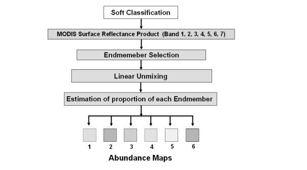
Spectral mixture analysis provides an efficient mechanism for the interpretation of remotely sensed multidimensional imagery. It aims to identify a set of reference signatures (endmembers) that can be used to model the reflectance spectrum at each pixel of the original image. These endmembers can be directly extracted from the image using techniques like PPI, scatter plot etc. Thus, the modelling is carried out as a linear combination of a finite number of ground components. The modelling can be used to estimate the proportion of each endmember is a single pixel and to produce an abundance map pertaining to each class.

Figure 4. 3 : Overall methodology of linear unmixing process.