Hard Classification Techniques

Land cover analysis is the first level of classification that helps in identifying land cover in terms of vegetation and non vegetation. This is done by slope based and distance based indices depending on the region (arid versus vegetated area). The slope based and the distance based vegetation indices (VIs) help in land cover analysis depending on the extent of vegetation and soil in a region. The slope-based VIs are simple arithmetic combinations that focus on the contrast between the spectral response patterns of vegetation in the red and near-infrared portions of the electromagnetic spectrum. The distance-based group measures the degree of vegetation present by gauging the difference of any pixel's reflectance from the reflectance of bare soil.

Different feature types lead to different combinations of DNs (Digital Numbers) based on their inherent spectral reflectance and emittance properties. The term pattern refers to the set of radiance measurements obtained in the various wavelength bands for each pixel. Spectral pattern recognition refers to the family of classification procedures that utilizes this pixel-by-pixel spectral information as the basis for automated image classification and, indeed, the spectral pattern present within the data for each pixel is used as the numerical basis for categorization [19]. The overall objective of image classification procedures is to automatically categorise all pixels in an image into land cover classes or themes. Spectral Classification can be broadly categorised in to two types: Supervised classification and Unsupervised Classification.

This chapter discusses the most commonly used Vegetation Index; NDVI (Normalized Difference Vegetation Index) for land cover mapping, and then highlights the various hard classification techniques including Supervised and Unsupervised (K-means algorithm) that are used for land cover mapping. A comparison of the advantages and the disadvantages of the supervised and unsupervised approach is summarised and the chapter concludes with a brief discussion on the accuracy assessment.

3.1 NDVI time series analysis

Vegetated areas have a relatively high near-IR (Infrared) reflectance and low visible reflectance. Due to this property of the vegetation, various mathematical combinations of the NIR and the Red band have been found to be sensitive indicators of the presence and condition of green vegetation. These mathematical quantities are thus referred to as vegetation indices [19]. The most commonly used of these indices is the NDVI (Normalized Difference Vegetation Index) that is computed using the formula (NIR-RED)/(NIR+RED). It separates green vegetation from its background soil brightness and retains the ability to minimize topographic effects while producing a measurement scale ranging from –1 to +1 with NDVI-values £ 0 representing no vegetation. The NDVI is sensitive to the presence of vegetation, since green vegetation usually decreases the signal in the red due to chlorophyll absorption and increases the signal in the NIR wavelength due to light scattering by leaves [62].

The success of the NDVI to monitor vegetation variations on a large scale, despite the presence of atmospheric effects [63], [64] and [65] is due to the normalisation involved in its definition. The normalization reduces the effect of degradation of the satellite calibration from 10% - 30% for a single channel to 0-6% for the normalized index [66] and [67]. The effect of the angular dependence of the surface bidirectional reflectance and of the atmospheric effects is also reduced significantly in the normalized index [66], [69] and [70]. The effect of scattering and absorption by atmospheric aerosol and gases (mainly water vapour) and by undetected clouds is reduced significantly in the compositing of the NDVI from several consecutive images, choosing a value that corresponds to the maximum vegetation index for each pixel [69], [70] and [71].

The potential of computing NDVI has created great interest to study global biosphere dynamics [72]. It is preferred to the simple index for global vegetation monitoring because the NDVI helps compensate for changing illumination conditions, surface slope, aspect and other extraneous factors. Numerous investigators have related the NDVI to several vegetation phenomena. These phenomena have ranged from vegetation seasonal dynamics at global and continental scales, to tropical forest clearance, leaf area index measurement, biomass estimation, percentage ground cover determination and FPAR (fraction of absorbed photosynthetically active radiation). In turn, these vegetation attributes are used in various models to study photosynthesis, carbon budgets, water balance and related processes [19].

Many researchers have attempted to produce regional-scale land cover datasets using coarse spatial-resolution, high temporal-frequency data from the AVHRR instrument aboard the NOAA series of meteorological satellites. Almost without exception, these efforts have involved the conversion of AVHRR bands 1 and 2 to Normalised Difference Vegetation Index (NDVI) values. A registered time series of NDVI images is then composited so that, for every pixel location, the maximum NDVI value encountered throughout the compositing period is output. The compositing procedure tends to select against measurements that are strongly influenced by atmospheric and aerosol scattering. These measurements have reduced NDVI values due to differential scattering effects in red and near-infrared bands. Cloud-contaminated measurements also produce lower NDVI values, as clouds reflect strongly in both the red and near-infrared wave bands. The compositing of NDVI values further reduces the variability associated with changing view and illumination geometry [68], although measurements near the forward-scattering direction tend to have slightly higher NDVI values and will thus be preferentially selected. Compositing periods are chosen based on a trade-off between the expected frequency of changes in vegetation and the minimum length of time necessary to produce cloud-free images.

NDVI generally quantifies the biophysical activity of the land surface and, as such, does not provide land cover type directly. However, a time series of NDVI values can separate different land cover types based on their phenology, or seasonal signals ( e.g . [73]) . Reed et al . [74] and DeFries et al . [75] have developed and used multitemporal phenological metrics to derive land cover classifications from AVHRR data. Lambin and Ehrlich ( [76], [77]) have found that using a time series of the ratio of surface temperature to NDVI provides a more stable classification than NDVI alone, primarily by isolating interannual climatological variability.

Townshend [78] performed supervised classifications on composited NDVI GAC (Global Area Coverage) data for South America. While they did not validate their results with test data, they found that accuracy for the training sites improved substantially with the increase in the number of images included in the time series. Koomanoff [79] used annually-integrated NDVI values to generate a global vegetation map using NOAA's Global Vegetation Index product (GVI). This work represents nine vegetation types and does not rely on the seasonality of the NDVI. Lloyd [80] employed a binary classifier based on summary indices derived from a time series of NDVI data. These phytophenological variables included the date of the maximum photosynthetic activity, the length of the growing season, and the mean daily NDVI value. The variables were fed through a binary decision tree classifier that stratified pixels based first on the date of the maximum NDVI, then the length of the growing season, and finally on the mean daily NDVI.

A coarse-resolution global land surface parameter database was generated as an activity of the International Satellite Land Surface Climatology Project (ISCLSCP) [81]. The database includes land cover classes, absorbed fraction of photosynthetically-active radiation (FPAR), leaf area index (LAI), roughness length, and canopy greenness fraction, along with data on global meteorology, soils and hydrology. The spatial scale of the database is 1 degree by 1 degree. Variables such as FPAR, LAI and canopy greenness fraction are derived from 8-km composited AVHRR NDVI data. The land cover classification is based on a spatial aggregation of the 8-km data to one degree followed by supervised classification of the temporal patterns in NDVI [18].

Loveland's efforts were expanded under the auspices of the IGBP-DIS (International Geosphere Biosphere Programme-Data and Information System), based on a global database of 1-km AVHRR observations received during the period April 1992 through September 1993 [82] and [83]. These have been assembled and 10-day composited at the EROS Data Center (EDC). The 10-day composite AVHRR data were then monthly composited using maximum NDVI to remove cloud and topographic effects and extreme off-nadir pixels [68] and [84] , as well as scan angle dependence of radiance [85]. The use of the monthly-composited AVHRR data may be problematic [68]. An analysis by Zhu and Yang [86] determined that compositing was biased towards selecting off-nadir pixels, especially in forward-scanning views in winter months in the northern hemisphere. As with any large-area projection, they also found that the effective mapping unit was geographically variable, in this case due to the Goode's homolosine projection system and resampling methods. Lack of sensor calibration confuses the temporal trajectory of the multitemporal NDVI signal [87]. Temporal smoothing or generalization might enhance the meaning of the temporal signal [98].

The global NDVI data provided a multitemporal database for land cover classification using an unsupervised clustering and labeling approach. The global IGBP product has recently undergone validation based on a global network of some 400 stratified samples that were characterized using finer-resolution Landsat TM and SPOT-XS data following an expert interpretation approach [1].

In supervised classification, the pixel categorization process is done by specifying the numerical descriptors of the various land cover types present in a scene. It involves three steps –

(1) training stage: identifying representative training areas and developing a numerical description of the spectral attributes of each land cover type in the scene, known as training set ,

(2) classification stage: each pixel in the image data set is categorized into the land cover class it most closely resembles, and

(3) output stage: the process consists of a matrix of interpreted land cover category types [19].

The following subsections discuss the classification strategies that use the ‘ training set ' descriptions of the category spectral response patterns as interpretation keys by which pixels of unidentified cover type are categorised into their appropriate classes.

The maximum likelihood classifier quantitatively evaluates both the variance and covariance of the category spectral response patterns when classifying an unknown pixel. It is assumed that the distribution of the cloud of points forming the category training data is Gaussian (normally distributed). This assumption of normality is generally reasonable for common spectral response distributions. Under this assumption, the distribution of a category response pattern can be completely described by the mean vector and the covariance matrix. With these parameters, the statistical probability of a given pixel value being a member of a particular land cover class can be computed. The resulting bell-shaped surfaces are called probability functions, and there is one such function for each spectral category [19] .

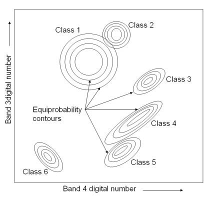
The probability density functions are used to classify an unidentified pixel by computing the probability of the pixel value belonging to each category. After evaluating the probability in each category, the pixel is assigned to the most likely class (highest probability value) or can be labelled as “unknown” if the probability values are all below a threshold set by the analyst. Essentially, the maximum likelihood classifier delineates ellipsoidal “equiprobability contours” through a scatter diagram as shown in figure 3.1 [19] .

Figure 3. 1 : Equiprobability contours defined by a maximum-likelihood classifier.

An extension of the maximum likelihood approach is the Bayesian classifier . This technique applies two weighting factors to the probability estimate. First, the “a priori probability”, or the anticipated likelihood of occurrence for each class in the given scene is determined. Secondly, a weight associated with the “cost” of misclassification is applied to each class. Together, these factors act to minimize the “cost” of misclassification, resulting in a theoretically optimum classification. Most maximum likelihood classifications are performed assuming equal probability of occurrence and cost of misclassification for all classes. If suitable data exist for these factors, the Bayesian implementation of the classifier is preferable [19] . For a mathematical description of Bayes' Classification see Annexure B.

Drawback of the GMLC Technique

The successful application of MLC is dependent upon having delineated correctly the spectral classes in the image data of interest. This is necessary since each class is to be modelled by a normal probability distribution, as discussed earlier. If a class happens to be multimodal, and this is not resolved, then clearly the modelling cannot be very effective [45] . The drawback of maximum likelihood classification is the large number of computation required to classify each pixel. This is particularly true when either a large number of spectral channels are involved or a large number of spectral classes must be differentiated. In such cases, the maximum likelihood classifier is much slower computationally than other algorithms [19]. In addition, MLC requires that every training set must include at least one more pixel than there are bands in the sensor and more often it is desirable to have the number of pixels per training set be between 10 times and 100 times as large as the number of sensor bands, in order to reliably derive class-specific covariance matrices.

To increase the efficiency, of the maximum likelihood classifiers, the category identity for all possible combinations of digital numbers occurring in an image is determined in advance of actually classifying the image. Hence, the complex statistical computation for each combination is only made once. The categorization of each pixel in the image is then simply a matter of indexing the location of its multichannel gray level. Another means of optimizing the implementation of the MLC is to use some data dimensionality reduction technique [19].

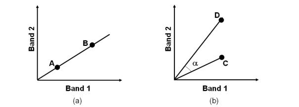
In N dimensional multi-(or hyper-) spectral space a pixel vector x has both magnitude (length) and an angle measured with respect to the axes that defines the coordinate system of the space [45]. In the Spectral Angle Mapper (SAM) technique for identifying pixel spectra only the angular information is used. SAM is based on the idea that an observed reflectance spectrum can be considered as a vector in a multidimensional space, where the number of dimensions equals the number of spectral bands. If the overall illumination increases or decreases (due to the presence of a mix of sunlight and shadows), the length of this vector will increase or decrease, but its angular orientation will remain constant. Figure 3.2 (a) shows that for a given feature type, the vector corresponding to its spectrum will lie along a line passing through the origin, with the magnitude of the vector being smaller (A) or larger (B) under lower or higher illumination, respectively. Figure 3.2 (b) shows the comparison of the vector for an unknown feature type (C) to a known material with laboratory-measured spectral vector (D), the two features match if the angle ‘ a ' is smaller than a specified tolerance value [89].

Figure 3. 2 : Spectral Angle Mapping concept. (a) For a given feature type, the vector corresponding to its spectrum will lie along a line passing through the origin, with the magnitude of the vector being smaller (A) or larger (B) under lower or higher illumination, respectively. (b) When comparing the vector for an unknown feature type (C) to a known material with laboratory-measured spectral vector (D), the two features match if the angle ‘ a ' is smaller than a specified tolerance value. (After Kruse et al., 1993) [34].

To compare two spectra, such as an image pixel spectrum and a library reference spectrum, the multidimensional vectors are defined for each spectrum and the angle between the two vectors is calculated. Smaller angles represent closer matches to the reference spectrum. If this angle is smaller than a given tolerance level, the spectra are considered to match, even if one spectrum is much brighter than the other (farther from the origin) overall [19]. Pixels further away than the specified maximum angle threshold are not classified. The reference endmember spectra used by SAM can come from ASCII files, spectral libraries, statistics files, or can be extracted directly from the image.

Girouard et al. [90] validated the SAM algorithm for geological mapping in Central Jebilet Morocco and compared the results between high and medium spatial resolution sensors, such as Quickbird and Landsat TM, respectively. The result showed that SAM of TM data can provide mineralogical maps that compare favourably with ground truth and known surface geology maps. Even though, Quickbird has a high spatial resolution compared to TM; its data did not provide good results for SAM because of the low spectral resolution.

Drawback of SAM

SAM technique fails if the vector magnitude is important in providing discriminating information, which happens in many instances [45]. However, if the pixel spectra from the different classes are well distributed in feature space there is a high likelihood that angular information alone will provide good separation. This technique functions well in the face of scaling noise.

To overcome difficulties in conventional digital classification that uses the spectral characteristics of the pixel as the sole parameter in deciding to which class a pixel belongs to, new approaches such as Neural Networks (NN) are being used. They can be used to perform traditional image classification tasks [91] and are also increasingly used for more complex operations such as spectral mixture analysis [92]. For image classification, neural networks do not require that the training class data have a Gaussian statistical distribution, a requirement that is held by maximum-likelihood algorithms. This allows neural networks to be used with a much wider range of types of input data than could be used in a traditional maximum-likelihood classification process. In addition, once they have been fully trained, neural networks can perform image classification relatively rapidly, although the training process itself can be quite time consuming. NN systems are “self-training” in that they adaptively construct linkages between a given pattern of input data and particular outputs [19].

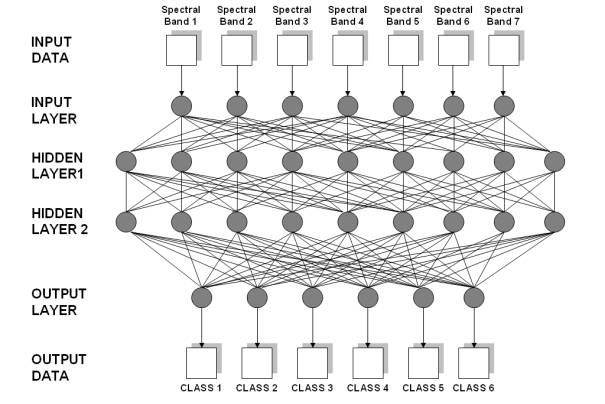
A NN consists of a set of three or more layers, each made up of multiple nodes. These nodes are somewhat analogous to the neurons in a biological neural network and thus are sometimes referred to as “ neurons” . The network's layers include an input layer, an output layer, and one or more hidden layers. The nodes in the input layer represent variables used as input to the neural network. Typically, these might include spectral bands from a remotely sensed image, textural features or other intermediate products derived from such images, or ancillary data describing the region to be analysed. The nodes in the output layer represent the range of possible output categories to be produced by the network. If the network is being used for image classification, there will be one output node for each class in the classification system [19].

Between the input and output layers are one or more hidden layers. These consist of multiple nodes, each linked to many nodes in the preceding layer and to many nodes in the following layer. These linkages between nodes are represented by weights, which guide the flow of information through the network. The number of hidden layers used in a neural network is arbitrary. An increase in the number of hidden layers permits the network to be used for more complex problems but reduces the network's ability to generalize, and increases the time required for training [19].

Figure 3.3 shows an example of a neural network that is used to classify land covers based on a combination of spectral information. There are seven nodes in the input layer (Spectral Bands 1 to 7). After the input layer, there are two hidden layers, each with nine nodes. Finally, the output layer consists of six nodes, each corresponding to a land cover class. When given any combination of input data, the network produces the output class that is most likely to result from that set of inputs, based on the network's analysis of previously supplied data. Applying a NN to image classification makes use of an iterative training procedure in which the network is provided with matching sets of input and output data. Each set of input data represents an example of a pattern to be learned, and each corresponding set of output data represents the desired output that should be produced in response to the input. During the training process the network autonomously modifies the weights on the linkages between each pair of nodes in such a way as to reduce the discrepancy between the desired output and the actual output [19].

Figure 3. 3 : Example of an artificial neural network with one input layer, two hidden layers and one output layer [19].

The bulk of neural network classification work in remote sensing has used multiple layer feed-forward networks that are trained using the back-propagation algorithm based on a recursive learning procedure with a gradient descent search [4]. However, this training procedure is sensitive to the choice of initial network parameters and to over-fitting [93]. The use of Adaptive Resonance Theory (ART) can overcome these problems. Networks organized on the ART principle are stable as learning proceeds, while at the same time they are flexible enough to learn new patterns and improves especially the overall accuracy of classification of multi-temporal data sets [94], [93]. Recent MODIS-based land cover classification used a class of ART NN called fuzzy ARTMAP, for classification, change detection and mixture modelling. Many studies based on ARTMAP have been directed toward recognition of land cover classes, which have ranged from broad life-form categories [95] to floristic classes [96].

Remotely sensed datasets processed by NN-based classifiers have included images acquired by the Landsat Multispectral Scanner (MSS) [97], [98], Landsat TM [99], Synthetic Aperture Radar [100], SPOT HRV [101], AVHRR [94] and aircraft scanner data [102]. A number of these studies have also included ancillary data e.g ., topography [103] and texture [104]. Most use a supervised approach, but unsupervised classification using self-organizing neural networks has also been attempted [100]. In all cases, the neural network classifiers have proven superior to conventional classifiers, often recording overall accuracy improvements in the range of 10-20 percent. As the number of successful applications of neural network classification increases, it is increasingly clear that neural network-based classification can produce more accurate results than conventional approaches for remote sensing.

Summary of Neural Network

While there are a variety of different NN models, most remote sensing applications have used a supervised, feedforward structure employing a backpropagation algorithm that adjusts the network weights to produce convergence between the network outputs and the training data. In overview, the NN classifier is composed of layers of “neurons” that are interconnected through weighted synapses. The first layer consists of the classification input variables and the last layer consists of a binary vector representing the output classes. Intermediate, “hidden” layers provide an internal representation of neural pathways through which input data are processed to arrive at output values or conclusions.

In a supervised approach, the neural network is trained on a dataset for which the output classes are known. In this process, the input variables are fed forward through the network to produce an output vector. During a following backpropagation phase, the synapse weights are adjusted so that the network output vector more closely matches the desired output vector, which is a binary-coded representation of the training class. The network weights, or processing element responses, are adjusted by feeding the summed squared errors from the output layer back through the hidden layers to the input layer. In this fashion, the network cycles through the training set until the synapse weights have been adjusted so that the network output has converged, to an acceptable level, with the desired output. The trained neural network is then given new data, and the internal synapses guide the processing flow through excitement and inhibition of neurons. This results in the assignment of the input data to the output classes.

Advantages and drawbacks of Neural Networks

•  Neural network classifiers, without any priori assumptions about data distributions, are able to learn nonlinear and discontinuous patterns in the distribution of classes.

•  Neural networks can readily accommodate auxiliary data such as textural information, slope, aspect and elevation, and

•  Neural networks are quite flexible and can be adapted to improve performance for particular problems [1].

The back propagation NN is not guaranteed to find the ideal solution to a particular problem. During the training process the network may develop in such a way that it becomes caught in a “local minimum” in the output error field, rather than reaching the absolute minimum error. Alternatively, the network may begin to oscillate between two slightly different states, each of which results in approximately equal error [105]. A variety of strategies have been proposed to help push neural networks out of these pitfalls and enable them to continue development toward the absolute minimum error. Again, the use of ANN in image classification is the subject of continuing research [19].

3.2.4 Decision Tree Approach

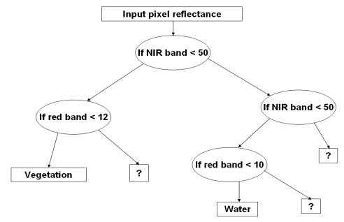
Decision tree approach is a non-parametric classifier and an example of machine learning algorithm. It involves a recursive partitioning of the feature space, based on a set of rules that are learned by an analysis of the training set. A tree structure is developed where at each branching a specific decision rule is implemented, which may involve one or more combinations of the attribute inputs. A new input vector then “travels” from the root node down through successive branches until it is placed in a specific class [4].

The thresholds used for each class decision are chosen using minimum entropy or minimum error measures. It is based on using the minimum number of bits to describe each decision at a node in the tree based on the frequency of each class at the node. With minimum entropy, the stopping criterion is based on the amount of information gained by a rule (the gain ratio) [4].

A decision tree is composed of a root node, a set of interior nodes, and terminal nodes, called “leaves”. The root node and interior nodes, referred to collectively as non-terminal nodes, are linked into decision stages. The terminal nodes represent final classification. The classification process is implemented by a set of rules that determine the path to be followed, starting from the root node and ending at one terminal node, which represents the label for the object being classified. At each non-terminal node, a decision has to be taken about the path to the next node. Figure 3.4 illustrates a simple decision tree using pixel reflectance as input [4].

Figure 3. 4 : Example of Decision Tree

• If there are k classes denoted { C1, C2,….Ck }, and a training set, T , then
• If T contains one or more objects which all belong to a single class Cj , then the decision tree is a leaf identifying class Cj .
• If T contains no objects, the decision tree is a leaf determined from information other than T .
• If T contains objects that belong to a mixture of classes, then a test is chosen, based on a single attribute that has one or more mutually exclusive outcomes {O1, O2,…On} . T is portioned into subsets T1, T2,…Tn , where Ti contains all the objects in T that have outcome Oi of the chosen test. The same method is applied recursively to each subset of training objects to build the decision tree.

An attempt was made by [106] to classify the agricultural fields under different manure/fertilizer application strategies. During the summer of 2000, airborn hyperspectral data were collected three times at two field sites in south-western Quebec, Canada. One field site contained plots that were amended with manure treatments and planned with maize and soya beans. The second field site contained plots that received chemical fertilizers and were planted with maize. Reflectances of 71 wave bands of hyperspectral data were collected and the decision tree algorithm of data mining technology was used to distinguish between manure and chemical fertilizer treatments. The decision tree approach divided the data to reduce the deviance, and classified them into the pre-defined categories as many tree branches. The success of the classification rate was reported to be high.

A decision tree classifier was used for land use classification using Landsat-7 ETM+ data for an agricultural area near Littleport (Cambridgeshire), UK, for the year 2000. A field study was carried out to collect ground truth information about the various land use classes. Six land use classes (wheat, sugar beet, potatoes, peas, onions and lettuce) were selected for classification, and a univariate decision tree classifier was used for labelling the image pixels. The results of the study suggest that the decision tree classifier performs well. The boosting technique improved the classification accuracy of a base classifier and the classification accuracy increased [107].

Advantages of Decision Tree Approach

The advantages of decision tree classifier over traditional statistical classifier include its simplicity, ability to handle missing and noisy data, and non-parametric nature. Decision trees are not constrained by any lack of knowledge of the class distributions. It can be trained quickly, takes less computational time.

The strength of supervised classification based upon the maximum likelihood procedure is that it minimises classification error for classes that are distributed in a multivariate normal fashion. Moreover, it can label data relatively quickly. Its major drawback lies in the need for training data and the need to have delineated unimodal spectral classes beforehand. This, however, is a task that can be handled using clustering, based upon a representative subset of image data. Used for this task, unsupervised classification performs the valuable function of identifying the existence of all spectral classes, yet it is not expected to perform the entire classification.

Unsupervised Classification is an analytical procedure based upon clustering algorithms. Unsupervised classifiers do not utilize training data as the basis for classification. Rather they examine the unknown pixels in an image and aggregate them into a number of classes based on the natural groupings or clusters present in the image values. The basic premise is that the values within a given cover type should be close together in the measurement space, whereas data in different classes should be comparatively well separated. The classes that result from unsupervised classification are spectral classes. Thus, here spectrally separable classes are determined and then their informational utility is defined [19]. The identification of classes of interest against reference data is often more easily carried out when the spatial distribution of spectrally similar pixels has been established in the image data. This is an advantage of unsupervised classification and the technique is therefore a convenient means by which to generate signatures for spatially elongated classes such as rivers and roads [45] . Consequently, it is not unusual in practice to iterate over sets of steps as experience is gained with the particular problem at hand [45] . A final point that must be taken into account when contemplating unsupervised classification via clustering is that there is no facility for including prior probabilities of class membership. By comparison the decision functions for maximum likelihood classification can be biased by previous knowledge or estimates of class membership [45] .

Users of remotely sensed data can only specify the information classes. Occasionally it might be possible to guess the number of spectral classes in a particular information class but, in general, the user would have little idea of the number of distinct unimodal groups that the data falls into in multispectral space. Clustering procedures can be used for that purpose. These are methods that have been applied in many data analysis fields to enable inherent data structures to be determined. Clustering partitions the image data into a number of spectral classes, and then labels all pixels of interest as belonging to one of those spectral classes, although the labels are purely nominal (e.g. A, B, C, …., or class1, class 2, …….) and are as yet unrelated to ground cover types. Clustering is also the basis for unsupervised classification. The classes are preferably unimodal; however, if simple unsupervised classification is of interest, this is not essential [45] .

Clustering techniques fall into a group of undirected data mining tools [108]. The goal of clustering is to discover structure in the data as a whole. There is no target variable to be predicted and thus no distinction is being made between independent and dependent variables. Clustering techniques are used for combining observed examples into clusters (groups) which satisfy two main criteria:

•  Each group or cluster is homogeneous; i.e. examples that belong to the same group are similar to each other.

•  Each group or cluster should be different from other cluster, i.e. examples that belong to one cluster should be different from the examples of other clusters.

Depending on the clustering technique, clusters can be expressed in different ways:

•  Identified clusters may be exclusive, so that any example belongs to only one cluster.

•  They may be overlapping, an example may belong to several clusters.

•  They may be probabilistic, whereby an example belongs to each cluster with a certain probability.

•  Clusters might have hierarchical structure, having crude division of examples at highest level of hierarchy, which is then refined to sub-clusters at lower levels.

Clustering is first employed to determine the spectral classes, using a subset of the image data. It is therefore recommended that about 3 to 6 small regions, or so-called candidate clustering areas, be chosen for this purpose. These should be well spaced over the image and located such that each one contains several of the cover types (information class) of interest and such that all cover types are represented in the collection of clustering areas. An advantage in choosing heterogeneous regions to cluster, as against apparently homogeneous training areas used in supervised classification, is that mixture pixels lying on class boundaries will be identified as legitimate spectral classes [45] .

If an iterative clustering procedure is used, the analyst will have to pre-specify the number of clusters expected in each candidate area. Experience has shown that, on average, there are about 2 to 3 spectral classes per information class. This number should be chosen with a view of removing or rationalising unnecessary clusters at a later stage. It is useful to cluster each region separately as this saves computation, and produces cluster maps within those areas with more distinct class boundaries than would be the case if all regions were pooled beforehand [45] .

Most clustering procedures in remote sensing generate the mean vector and covariance matrix for each cluster found. Accordingly, separability measures can be used to assess whether feature reduction is necessary or whether some clusters are sufficiently similar spectrally and should be merged. These are only considerations of course if the clustering is generated on a sample of data, with a second phase used to allocate all image pixels to a cluster. Feature selection would be performed between the two phases [45] .

Clustering sorts the image into unknown classes [45] . Following this sorting of the data space by clustering, the clusters or spectral classes are associated with information classes – i.e. ground cover types – by the analyst, using available reference data. Thus a posteriori identification may need to be performed explicitly only for classes of interest. The other classes will have been used by the algorithm to ensure good discrimination but will remain labelled only by arbitrary symbols rather than by class names [45] .

Decisions about merging can be made on the basis of separability measures. During the rationalisation procedure it is useful to be able to visualise the locations of spectral classes. For this a bispectral plot can be constructed. This bispectral plot is not unlike a two dimensional scatter plot view of the multispectral space in which the data appears. However, rather than having the individual pixels shown, the class or cluster means are located according to their spectral components. Sometimes, depending upon the cases in hand, the most significant pair of spectral bands would be chosen in order to view the relative locations of the cluster centres. In general, the choice of bands and combinations to use in a bi-spectral plot will depend on the sensor and application. Sometimes, several plots with different bands will give a fuller appreciation of the distribution of classes in feature space [45] . For a discussion on clustering criteria, please see Annexure B.

This algorithm has as an input, a predefined number of clusters (i.e., the K from its name. Means stands for an average, an average location of all the members of a particular cluster). When dealing with clustering techniques, one has to adopt a notion of a higher dimensional space, or space in which orthogonal dimensions are all attributes. The value of each attribute of an example represents a distance of the example from the origin along the attribute axes. Of course, in order to use this geometry efficiently, the values in the data set must all be numeric (categorical data must be transformed into numeric ones) and should be normalized in order to allow fair computation of the overall distances in a multi-attribute space.

The K-means algorithm is a simple, iterative procedure, in which a crucial concept is the one of “ centroid ”. Centroid is an artificial point in the space of records which represents an average location of the particular cluster. The coordinates of this point are averages of attribute values of all examples that belong to the cluster. The steps of the k-means algorithm are given below.

•  Select randomly k points (it can also be examples) to be the seeds for the centroids of k clusters.

•  Assign each example to the centroid closest to the example, forming in this way k exclusive clusters of examples.

•  Calculate new centroids of the clusters. For that purpose, average all attribute values of the examples belonging to the same cluster (centroid).

•  Check if the cluster centroids have changed their “coordinates”. If yes, start again from the step (ii). If not, cluster detection is finished and all examples have their cluster memberships defined.

Usually this iterative procedure of redefining centroids and reassigning the examples to clusters needs only a few iterations to converge. For a discussion on cluster detection see Annexure B.

To summarise, clustering techniques are used when there are natural grouping in a data set. Clusters should then represent groups of items that have a lot in common. Creating clusters prior to application of some other data mining technique might reduce the complexity of the problem by dividing the space of data set. This space partitions can be mined separately and such two steps procedure might give improved results as compared to data mining without using clustering.

The result of unsupervised classification is simply the identification of spectrally distinct classes in image data. Hence, proper interpretation of these spectral classes by analyst is required along with reference data to associate the spectral classes with the cover types of interest. This process, like the training set refinement step in supervised classification, can be quite involved [19].

Access to efficient hardware and software is an important factor in determining the ease with which an unsupervised classification can be performed. The quality of the classification still depends upon the analyst's understanding of the concepts behind the classifiers available and knowledge about the land cover types under analysis [19].

In contrast to the a priori use of analyst-provided information in supervised classification; unsupervised classification is a segmentation of the data space in the absence of any information provided by any analyst. Analyst information is used only to attach information class (or ground cover type, or map) labels to the segments established by clustering. Clearly this is an advantage of the approach. However, it is a time-consuming procedure computationally by comparison to techniques for supervised classification. Suppose a particular classification exercise involves N spectral bands and C classes. MLC requires CPN (N+1) multiplications where P is the number of pixels in the image segment of interest. By comparison, clustering of the data requires PCI distance measures for I iterations. Each distance calculation demands N multiplications (usually distance squared is calculated avoiding the need to evaluate the square root operation), so that the total number of multiplications for clustering is PCIN . Thus the speed comparison of the two approaches is approximately (N+1)/I for MLC compared with clustering. For example, for Landsat MSS data, therefore, in a situation where all 4 spectral bands are used, clustering would have to be completed within 5 iterations to be speed competitive with MLC.

Training of the classifier would add about a 10% loading to its time demand; however a significant time loading should also be added to clustering to account for the labelling phase. Often this is done by associating pixels with the nearest (Euclidean distance) cluster. However, sometimes Mahalanobis, or Maximum Likelihood distance labelling is used. This adds substantially to the cost of the clustering. Because of the time demand of clustering algorithms, unsupervised classification is often carried out with small image segments. Alternatively, a representative subset of data is used in the actual clustering phase in order to cluster or segment the feature space. That transformation is then used to assign all the image pixels to a cluster [45] .

When comparing time requirement of supervised and unsupervised classification it must be recalled that a large demand on user time is required in training a supervised procedure. This is necessary both determining training data and then identifying training pixels by reference to that data. The corresponding step in unsupervised classification is the a posteriori labelling of clusters. As noted earlier, data are only required for those classes of interest; moreover only a handful of labelled pixels is necessary to identify a class. By comparison, sufficient training pixels per class are required in supervised training to ensure reliable estimates of class signatures are generated [45]. Table 3.1 summarises the genesis, advantages and the disadvantages of all the techniques discussed above.

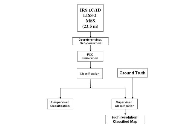
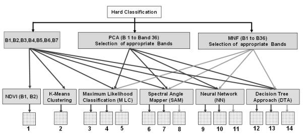
Figure 3.5, shows the steps for the LISS-3 preprocessing and classification. Figure 3.6 shows the overall methodology of the processing and hard classification of the MODIS bands 1 to 7, MODIS Principal Components and MODIS MNF components. A total of 14 different maps are produced from the MODIS classification which is discussed in Chapter 5.

Figure 3. 5 : LISS-3 Preprocessing and Classification.

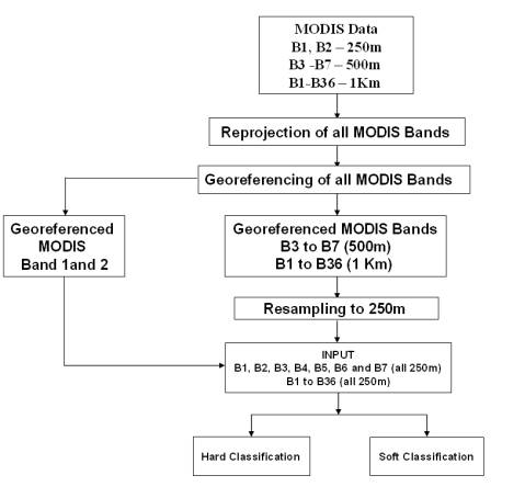
Figure 3. 6 : Processing and Hard Classification of MODIS data.

Statistical accuracy assessment of classified data is done to measure the agreement of classification with the field data (ground condition), and it constitutes an important stage in remote sensing data classification. One of the most common means of expressing classification accuracy is the preparation of a classification error matrix (also called confusion matrix or a contingency table). An adequate number of sample points representing different land cover categories are identified on the training data sets for accuracy estimation. A one-to-one comparison of the categories is mapped from all the training datasets and the classified image. Then based on the confusion matrix (errors of commission and omission), accuracy estimation in terms of producer's accuracy, user's accuracy, overall accuracy is subsequently calculated [109]. The Bradley-Terry (BT) model, which compares categories pairwise, was also attempted for accuracy assessment. The probability of one class over another class is estimated as well as the expected values of class pixels [110].

Error matrices compare, on a category by category basis, the relationship between the reference field data (ground truth) and the corresponding results of a classification. These are square matrices having equal number of rows, columns and categories (whose classification accuracy is being assessed). The major diagonal of the error matrix represents the properly classified land use categories. The non-diagonal elements of the matrix represent errors of omission or commission. Omission errors correspond to non diagonal column elements and commission errors are represented by non diagonal row elements. Overall accuracy is computed by dividing the total number of correctly classified pixels (sum of the elements along the major diagonal) by the total number of references pixels. Similarly, the accuracies of individual categories can be calculated by dividing the number of correctly classified pixels in each category by either the total number of pixels in the corresponding row or column. Producer's accuracies result from dividing the number of correctly classified pixels in each category (on the major diagonal) by the number of training set pixels used for that category (the column total). User's accuracies are computed by dividing the number of correctly classified pixels in each category by the total number of pixels that were classified in that category (the row total). This figure is a measure of commission error and indicates the probability that a pixel classified into a given category actually represents that category on the ground. Finally, the khat (KHAT or Kappa) statistics is a measure of the difference between the actual agreement between the reference data and an automated classifier and the chance agreement between the reference data and a random classifier.

k = observed accuracy – chance agreement /1 – chance agreement

This statistics serves as an indicator of the extent to which the percentage correct values of an error matrix are due to “true” agreement versus “chance” agreement. As true agreement observed approaches 1 and chance agreement approaches 0, k approaches 1. This is the ideal case. In reality, k usually ranges between 0 and 1 [19].

The results and findings of the above algorithms on MODIS data are discussed in Chapter 5 (Results) and their accuracy assessment is done in Chapter-6 (Accuracy Assessment).