Let the spectral classes for an image be represented by
![]()
where M is the total number of classes. In trying to determine the class or category to which a pixel at a location x belongs, it is strictly the conditional probabilities
![]()
that are of interest. The position vector x is a column vector of brightness values for the pixel. It describes the pixel as a point in multispectral space with co-ordinates defined by the brightness. The probability ![]() gives the likelihood that the correct class is
gives the likelihood that the correct class is ![]() for a pixel at a position x .
for a pixel at a position x .
Classification is performed according to
![]() -------------------------(equation 3.1)
-------------------------(equation 3.1)
i.e., the pixel at x belongs to class ![]() , if
, if ![]() is the largest. This intuitive decision rule is a special case of a more general rule in which the decision can be biased according to different degrees of significance being attached to different incorrect classifications [15].
is the largest. This intuitive decision rule is a special case of a more general rule in which the decision can be biased according to different degrees of significance being attached to different incorrect classifications [15].
Clustering implies a grouping of pixels in multispectral space. Pixels belonging to a particular cluster are therefore spectrally similar. In order to quantify this relationship it is necessary to device a similarity measure. Many similarity metrics have been proposed but those used commonly in clustering procedures are usually simple distance measures in multispectral space. The most frequently encountered are Euclidean distance and L1 (or interpoint) distance. If X 1 and X 2 are two pixels whose similarity is to be checked then the Euclidean distance between them is
D(x 1, x 2 ) = || x 1 - x 2 ||
= {(x 1 - x 2 )t (x 1 - x 2 )}1/2
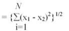
where, N is the number of spectral components. The L1 distance between the pixels is
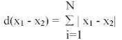
Clearly the later is computationally faster to determine [15]. However it can be seen as less accurate than the Euclidean distance measure. By using a distance measure it should be possible to determine clusters in data, as depicted in figure 1, so that once a candidate clustering has been found it is desirable to have a means by which the quality of clustering can be measured. The availability of such a measure should allow one cluster assignment of the data to be chosen over all others [15].
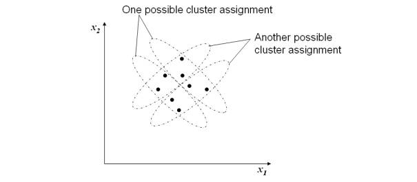
Figure 1: Two apparently acceptable clusterings of a set of two dimensional data.
A common clustering criterion or quality indicator is the sum of squared error (SSE) measure defined as
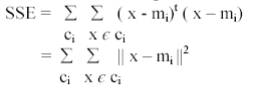
where, m i is the mean of the ith cluster and ![]() is a pattern assigned to that cluster. The outer sum is over all the clusters. This measure computes the cumulative distance of each pattern from its cluster centre for each cluster individually, and then sums those measures over all the clusters. If it is small the distances from patterns to cluster means are all small and the clustering would be regarded favourably. Another popular quality of clustering measures is to derive a within cluster scatter measure by determining the average covariance matrix of the clusters, and a between cluster scatter measure by looking at the means of the clusters compared with the global mean of the data. These two measures are combined into a single figure of merit as discussed in Duda and Hart (1973) [16] and Coleman and Andrews (1979) [17]. It can be shown that figures of merit such as these are essentially the same as the sum of squared error criterion.
is a pattern assigned to that cluster. The outer sum is over all the clusters. This measure computes the cumulative distance of each pattern from its cluster centre for each cluster individually, and then sums those measures over all the clusters. If it is small the distances from patterns to cluster means are all small and the clustering would be regarded favourably. Another popular quality of clustering measures is to derive a within cluster scatter measure by determining the average covariance matrix of the clusters, and a between cluster scatter measure by looking at the means of the clusters compared with the global mean of the data. These two measures are combined into a single figure of merit as discussed in Duda and Hart (1973) [16] and Coleman and Andrews (1979) [17]. It can be shown that figures of merit such as these are essentially the same as the sum of squared error criterion.
It is of interest to note that SSE has a theoretical minimum of zero, which corresponds to all clusters containing only a single data point. As a result, if an iterative method is used to seek the natural clusters or spectral classes in a set of data then it has a guaranteed termination point, at least in principle. In practice it may be too expensive to allow natural termination. Instead, iterative procedures are often stopped when an acceptable degree of clustering has been achieved. While the implementation of an actual clustering algorithm depend upon a progressive minimization (and thus calculation) of SSE for the evaluation of all candidate clusterings. For example, there are approximately C p /C! ways of placing P patterns into C clusters [15]. This number of SSE ( sum of squared error) values would require computation at each stage of clustering to allow a minimum to be chosen. Some of the clustering techniques that are often used are The Iterative Optimization (Migrating Means) Clustering Algorithm, a Single Pass Clustering Technique, Self-Organizing maps (Kohonen networks), Probabilistic Clustering Methods (Auto Class algorithm), Agglomerative Hierarchical Clustering, Clustering by Histogram peak Selection, K-Means Clustering etc. which are sophisticated and proficient [15] . The basics of the simplest of clustering methods namely K-means algorithm, which is used for data clustering is discussed in the next section. K-means algorithm is the one which is most widely used in the remote sensing application, when there is no prior knowledge about the data set.
Most of the issues related to automatic cluster detection are connected to the data mining project, or data preparation for their successful application.
Distance measure: Most clustering techniques use for the distance measure the Euclidean distance (square root of the sum of the squares of distances along each attribute axes). Non-numeric variables must be transformed and scaled before the clustering can take place. Depending on the transformation, the categorical variables may dominate clustering results or they may be even completely ignored.
Choice of the right number of clusters: If the number of clusters k in the k-means method is not chosen so to match the natural structure of the data, the results will not be good, as the clusters obtained may not be homogenous or two or more clusters may merge in one cluster. The proper way to alleviate this is to experiment with different values for k. In principle, the best k value will exhibit the smallest intra-cluster distances and largest inter-cluster distances. More sophisticated techniques measure these qualities automatically, and optimize the number of clusters in a separate loop.
Once the clusters are discovered they have to be interpreted in order to have some value for the data mining project. There are different ways to utilize clustering results:
• Cluster membership can be used as a label for the separate classification problem. Some descriptive data mining technique (like decision trees) can be used to find descriptions of clusters.
• Clusters can be visualized using 2D and 3D scatter graphs or some other visualization technique.
Differences in attribute values among different clusters can be examined, one attribute at a time.