| Back |
One of the challenging problems in processing high dimensional data with better spectral and temporal resolution is the computational complexity resulting from processing the vast amount of data volume [40]. This is particularly true for hyperspectral images containing numerous spectral bands. Preprocessing of hyperspectral imagery is required both for display and for proper band selection to reduce the data dimensionality and computational complexity.
When displaying multispectral data, both spatial dimensions and wavelength (x, y and l ) are generally used with three of the spectral bands written to the red, green and blue colour elements of the display device. Careful band selection is required in this process to ensure the most informative display. To enhance the richness of the displayed data, multispectral transformations such as principal components are useful.
2.1 The Challenges for Hyperspectral ProcessingHyperspectral data offers both challenges and opportunities for processing. The following section discusses briefly about calibration, atmospheric correction, radiometric correction and data normalisation of MODIS.
2.1.1 CalibrationCalibration is the conversion of DN into at-satellite radiances. There are three types of calibrations associated with MODIS data - (i) L1B Emissive Calibration [41], (ii) L1B Reflective Calibration [42], and (iii) Spectral Calibration [43]. For a brief discussion on each of these see Annexure A.
MODIS External Calibration Sources (ECs) - Two external calibration techniques that MODIS uses are views of the moon and deep space. The advantage of "looking" at the moon is that it enables MODIS to view an object that is roughly the same brightness as the Earth. Like the on-board Solar Diffuser, the moon is illuminated by the sun; however, unlike the Solar Diffuser or the Earth, the moon is not expected to change over the lifetime of the MODIS mission. "Looking" at the moon provides a second method for tracking degradation of the Solar Diffuser. "Looking" at deep space provides a photon input signal of zero, which is used as an additional point of reference for calibration [44].
Atmospheric constituents such as gases and aerosols have two types of effects on the radiance observed by a hyperspectral sensor, which is indicated in Figure 2.1.
Figure 2. 1 : Atmospheric effects influencing the measurement of reflected solar energy. Attenuated sunlight and skylight ( E ) is reflected from a terrain element having reflectance p . The attenuated radiance reflected from the terrain element ( pET/ ? ) combines with the path radiance ( Lp ) to form the total radiance ( L tot ) recorded by the sensor [19] .
The atmosphere affects the brightness or radiance, recorded over any given point on the ground in two almost contradictory ways, when a sensor records reflected solar energy. First it attenuates (reduces) the energy illuminating a ground object (and being reflected from the object) at particular wavelengths, thus decreasing the radiance that can be measured. Second, the atmosphere acts as a reflector itself, adding a scattered, extraneous path radiance to the signal detected by the sensor which is unrelated to the properties of the surface. By expressing these two atmospheric effects mathematically, the total radiance recorded by the sensor may be related to the reflectance of the ground object and the incoming radiation or irradiance using equation 2.1.
![]() --------------------- (equation 2.1)
--------------------- (equation 2.1)
where
Ltot = total spectral radiance measured by sensor
p = reflectance of object
E = irradiance on object, incoming energy
T = transmission of atmosphere
Lp =path radiance, from the atmosphere and from the object.
All these factors depend on wavelength. The irradiance (E) stems from two sources: directly reflected sunlight and diffuse skylight (sunlight scattered by the atmosphere). The relative dominance of sunlight versus skylight in a given image is strongly dependent on weather conditions. The irradiance varies with the seasonal changes in solar elevation angle and the changing distance between the earth and the sun [19].
The magnitude of absorption and scattering varies from place to place and time to time depending on the concentrations and particle sizes of the various atmospheric constituents. The end result is the raw radiance values observed by a hyperspectral sensor that cannot be directly compared to laboratory spectra or remotely sensed hyperspectral imagery acquired at other times or places. Before
such comparisons can be performed, an atmospheric correction process must be used to compensate for the transient effects of atmospheric absorption and scattering. These effects have not been particularly important in the processing and analysis of the multispectral data because of the absence of well defined atmospheric features and the use of average irradiance over each of the recorded wavelengths [45].
Hyperspectral data contain substantial amount of information about atmospheric characteristics at the time of image acquisition. In some cases, atmospheric models can be used with the image data themselves to compute quantities such as the total atmospheric column water vapour content and other atmospheric correction parameters. Alternatively, ground measurements of atmospheric transmittance or optical depth, obtained by instrument such as sunphotometers, may also be incorporated into the atmospheric correction methods.
Since hyperspectral data cover a whole spectral range from 0.4 to 2.4 m m, including water absorption features, and have high spectral resolution, a more systematic process is generally required, consisting of three possible steps:
• Compensation for the shape of the solar spectrum. The measured radiances are divided by solar irradiances above the atmosphere to obtain the apparent reflectances of the surface.
• Compensation for atmospheric gaseous transmittances and molecular and aerosol scattering. Simulating these atmospheric effects allows the apparent reflectances to be converted to scaled surface reflectances.
• Scaled surface reflectances are converted to real surface reflectances after consideration if any topographic effects. If topographic data are not available, real reflectance is assumed to be identical to scaled reflectance under the assumption that the surfaces of interest are Lambertian.
Procedures for solar curve and atmospheric modelling are incorporated in a number of models [46], including Lowtran 7 (Low Resolution Atmospheric Radiance and Transmittance), 5S Code (Simulation of the Satellite Signal in the Solar Spectrum) and Modtran 3 (The Moderate Resolution Atmospheric Radiance and Transmittance Model) [47]. ATREM (Atmosphere REMoval Program) [48], which is built upon 5S code, overcomes a difficulty with the other approaches in removing water vapour absorption features; water vapour effects vary from pixel to pixel and from time to time. In ATREM the amount of water vapour on a pixel by pixel basis is derived from AVIRIS data itself (although its technique may be independent of type of data) , particularly from the 0.94 m m to 1.14 m m water vapour features. A technique referred to as three-channel ratioing was developed for this purpose [46]. Other models like ACORN ( Atmospheric CORrection Now) account for accurate and proper cross-track spectral variation of push broom hyperspectral sensor (Hyperion, etc.). It also performs atmospheric correction of multispectral data with an independent water vapour image. FLAASH (Fast Line-of-Sight Atmospheric Analysis of Spectral Hypercubes) is an algorithm that handles data from a variety of hyperspectral sensors including AVIRIS, Hyperion, HyMap, etc., and supports off-nadir as well as nadir viewing. It also includes water vapour and aerosol retrieval and adjacency effect correction.
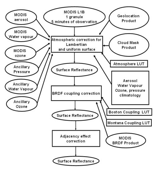
The atmospheric correction algorithm over land (the ACA, Atmospheric Correction Algorithm: Spectral Reflectances for MODIS [49] ) are applied to bands 1 7 of the MODIS data that uses aerosol and water vapour information derived from MODIS itself and takes into account the directional properties of the observed surface. The data being used in this research are therefore atmospherically corrected. The correction scheme includes corrections for the effects of atmospheric gases, aerosols, and thin cirrus clouds and is applied to all non cloudy L1B pixels that pass the L1B quality. Figure 2.2 gives an overview of the overall methodology and processing for atmospheric corrections [49]. For more relevant information on atmospheric correction see Annexure A.
Figure 2. 2 : Atmospheric correction processing thread flow chart [49].
The radiance measured by any given system over a given object is influenced by such factors as changes in scene illumination, atmospheric conditions, viewing geometry, and instrument response characteristics. For generating mosaics of satellite images taken in visible and NIR portion of the EM, it is usually necessary to apply a sun elevation correction and earth-sun-distance correction. The sun elevation correction accounts for the seasonal position of the sun relative to the earth. This is done by dividing each pixel value in a scene by the sine of the solar elevation angle for the particular time and location of the imaging. It normalises the image data acquired under different solar illumination angles by calculating pixel brightness values assuming the sun was at the zenith on each date of sensing. The earth-sun distance correction is applied to normalise for the seasonal changes in the distance between the earth and the sun.
Empirical Line procedure is one of the approaches of radiometric correction [50]. At least two spectrally uniform targets in the site of interest, one dark and one bright, are selected; their actual reflectances are then determined by field or laboratory measurements. The radiance spectra for each target are extracted from the image and then mapped to the actual reflectances using linear regression techniques. The gain and offset so-derived for each band are then applied to all pixels in the image to calculate their reflectances. While computational load is manageable with this method, field or laboratory data may not be available.
Another radiometric data processing activity in many quantitative applications is conversion of DNs to absolute radiance values. Such conversions are necessary when changes in the absolute reflectance of objects are to be measured over time using different sensors. Normally, detectors and data systems are designed to produce a linear response to incident spectral radiance. The absolute spectral radiance output of the calibration sources is known from prelaunch calibration and is assumed to be stable over the life of the sensor. Thus the onboard calibration sources form the basis for constructing the radiometric response function by relating known radiance values incident on the detectors to the resulting DNs.
The MODIS data being used in the research are radiometrically corrected and fully calibrated at the original instrument spatial and temporal resolution. These data are generated from Level-0 by appending geolocation and calibration data to the raw instrument data. The standard IRS 1C/1D LISS-3 MSS data procured from NRSA (National Remote Sensing Agency), Hyderabad is radiometrically and geometrically corrected. Normally all full scene, full scene Shift Along Track (SAT), sub-scenes and quadrant data products are supplied as standard data products [51].
There is special concern about atmospheric spectral transmittance and absorption characteristic and sensor calibration for hyperspectral imagery. This may be due to the following reasons:
• Hyperspectral sensors bands coinciding with narrow atmospheric absorption features or the edges of broader spectral features are affected by the atmosphere differently than the neighbouring bands.
• The band locations in imaging spectrometer systems are prone to small wavelength shifts under different operating conditions, particularly in airborne sensors.
A number of empirical techniques have been developed for the calibration of hyperspectral data that produce relative or absolute calibrations in an empirical way, without the explicit use of atmospheric data and models; for the reason they are more properly referred to as normalisation techniques, rather than calibration techniques. When detailed radiometric correction is not feasible (for example, because the necessary ancillary information is unavailable) normalisation is an alternative which makes the corrected data independent of multiplicative noise such as topographic and solar spectrum effects. This can be performed using Log Residuals [52], based on the relationship between radiance (raw data) and reflectance:
Xi, n = TiRinIn , i = 1, K ; n = 1, .. N ------------------- (equation 2.2)
where Xi, n is radiance for pixel i in wavelength n. Ti is the topographic effect, which is assumed constant for all wavelengths. Rin is the real reflectance for pixel i in wavelength band n. In is the (unknown) illumination factor, which is assumed independent of pixel. K and N are the total number of the pixels in the image and the total number of bands, respectively.
There are two steps which remove the topographic and illumination effects respectively. Xi, ncan be made independent of Ti and I n by dividing Xi, n by its geometric mean over all bands and then its geometric mean over all pixels. The result is not identical to reflectance but is independent of the multiplicative illumination and topographic effects present in the raw data. The procedure is carried out logarithmically so that the geometric means are replaced by arithmetic means and the final result obtained for the normalised data is
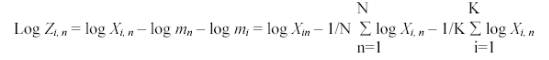 -----(equation 2.3)
The data produced by the imaging spectrometers is different from that of multispectral instruments due to its spectral characteristics. Firstly, the band selection for the display device is done in such a way so as to display maximum information. A two dimensional display using one geographical dimension and the spectral dimension can be created. These types of representation allows changes in spectral signatures with position (either along track or across track) to be observed. Usually, the greyscale is mapped to colour to enhance the interpretability of the displayed data. Secondly, choosing the most appropriate channels for processing is also not straight forward and requires careful selection to minimise the loss of the spectral benefits offered by this form of data gathering. A simple linear transformation such as the Principal Component Analysis or the Minimum Noise Fraction can be used for data dimensionality reduction [45].
Although, the hyperspectral data are both voluminous and multidimensional, nowadays with the availability of advanced computing systems that possess high speed processors and enormous storage power, data volume is no longer a constraint. The problem lies in the data redundancy that needs to be removed to obtain the bands with maximum information.
Much of the data does not add to the inherent information content for a particular application, even though it often helps in discovering that information; it contains redundancies. The data recorded by hyperspectral sensors often have substantial overlap of information content over the bands of data recorded for a given pixel. In such cases, not all of the data are needed to characterise a pixel properly, although redundant data may be different for different applications. Data redundancy can take two forms; spatial and spectral. Since hyperspectral imagery has more spectral concern, one way of viewing spectral redundancy in hyperspectral data is to form the correlation matrix for an image; the correlation matrix can be derived from the covariance matrix. High correlation between band pairs indicates high degree of redundancy. For example, PCT (Principal Component Transformation) assist in removing redundancy since decorrelation followed by a discarding of low variance components amounts to redundancy reduction [45].
Removal of least effective feature is referred to as feature selection , this being one form of feature reduction . The other is to transform the pixel vector into a new set of co-ordinates in which the features that can be removed are more evident [45]. Therefore, feature reduction, i.e., band reduction, has become a more significant part of image interpretation process.
Probably the most common approach is to employ some sort of linear transformation on the original dataset to produce a smaller set of factors or components [53], [54] and [55]. Most of the original variance is retained with a significant reduction in data volume [1].
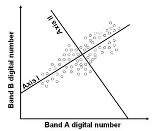
2.3.1 Principal Component Analysis (PCA)PCA transform multidimensional image data into a new, uncorrelated co-ordinate system or vector space. It produces a space in which the data have maximum variance along its first axis, the next largest variance along a second mutually orthogonal axis and so on (figure 2.3). Sometimes even the lower-order PC's may contain valuable information. The later principal components would be expected, in general, to show little variance. These could be considered therefore to contribute little to separability and could be ignored, thereby reducing the essential dimensionality of the classification space and thus improving classification speed [45]. Stated differently, the purpose of this process is to compress all the information contained in an original n band data set into fewer than n new bands or components . The components are then used in lieu of the original data [19]. These transformations may be applied as a preprocessing procedure prior to automated classification process of the data. Fundamentals and mathematical description of PCA are given in Annexure A.
Figure 2. 3 : Rotated coordinate axes in PCA [19].
This transformation is mainly used to reduce the dimensionality of hyperspectral data before performing the data fusion. It was first developed as an alternative to PCA for the airborne Thematic Mapper (ATM) 10- band sensor [56]. It is defined as a two-step cascaded PCA [57]. The first step, based on an estimated noise covariance matrix, is to decorrelate and rescale the data noise, where the noise has unit variance and no band-to-band correlations. The next step is a standard PCA of the noise-whitened data.
The MNF transformation is a linear transformation related to PC that orders the data according to signal-to-noise-ratio. It determines the inherent dimensionality of the data, segregates noise in the data and reduces the computational requirements for subsequent processing. It partitions the data space into two parts: one associated with large eigenvalues and coherent eigenimages, and a second with near-unity eigenvalues and noise-dominated images. By using only the coherent portions in subsequent processing, the noise is separated from the data, thus improving spectral processing results [58].
This transformation is equivalent to principal components when the noise variance is the same in all bands [56]. By applying the MNF to the Geophysical and Environment Research (GER) 64-band data, the results demonstrated the effectiveness of this transformation for noise adjustment in both the spatial and spectral domains [59].
Although PCA can efficiently compress hyperspectral data into a few components, this high concentration of total covariance only in the first few components inevitably results from part of the noise variance [56], [59] and [60]. The special capability image quality with increasing component number cannot be accomplished easily using other techniques, such as PCA and factor analysis. MNF, however, can help in this regard [61].