| Back |
Land cover describes the physical state of the earth's surface and immediate surface in terms of the natural environment (such as vegetation, soils, earth's surfaces and ground water) and the man-made structures (e.g. buildings). These land cover features have been classified using the remotely sensed satellite imagery of different spatial, spectral and temporal resolutions. Land cover analysis using high spectral resolution has several advantages, since it aids in numerous mapping applications such as soil types, species discrimination, mineral mapping etc. Hyperspectral data having numerous contiguous bands has high spectral resolution. Hyperspectral data processing possesses both challenges and opportunities for land cover mapping. Land cover mapping can be performed using various algorithms by processing the remotely sensed data into different themes or classes. The present research aims at comparing the results obtained from various classification algorithms using hyperspectral data for land cover mapping.
Land cover refers to what is actually present on the ground and may also contain an ecological description. It provides the ground cover information for baseline thematic maps. In contrast, land use refers to the various applications and the context of its use. Land use itself is the human employment of a land-cover type. It involves both the manner in which the biophysical attributes of the land are manipulated and the intent underlying that manipulation, the purpose for which the land is used. Identifying, delineating and mapping land cover on temporal scale provides an opportunity to monitor the changes, which is important for natural resource management and planning activities.
Land cover changes induced by human and natural processes play a major role in global as well as at regional scale patterns of the climate, hydrology and biogeochemistry of the earth system. Although the oceans are the major driving force for the earth's physical climatology, the land surface has considerable control on the planet's biogeochemical cycles, which in turn significantly influence the regional climate system through the radiative properties of green house gases and reactive species [1]. Terrestrial ecosystems exert considerable control on the planet's biogeochemical cycles, which in turn significantly influence the climate system [2]. Further, variations in topography, vegetation cover and other physical characteristics of the land surface influence surface-atmosphere fluxes of sensible heat, latent heat, and momentum, which in turn influence weather and climate [3] .
Land cover mapping employing moderate to coarse resolution datasets often in tandem with ancillary databases have been reported from different parts of the world at regional scale. The National Mapping program, a component of the U.S. Geological Survey (USGS), mapped land cover of the United States based on aerial photography acquired by NASA (National Aeronautics and Space Administration) and the USGS during 1970's and 1980's. The data were manually interpreted and land cover polygons were compiled onto 1:250, 000 base USGS maps. The Anderson hierarchical scheme used with this data had nine categories and several detailed level 2 classes [4].
Compilation of a 1:1 million scale atlas of Land cover Map as a first hand map for 1991 covering the entire territory of China was done based on field surveys, satellite images and aerial photos; classes were regrouped into 20 major land-use/land cover classes in the digital map [5]. Another database of China, the Temperate East Asia Land-Cover Database (TEAL) used 1992 NOAA (National Oceanic & Atmospheric Administration)-AVHRR (Advanced Very High Resolution Radiometer) 1-km remote sensing information and existing land cover maps developed using traditional and geographical techniques that involved extensive manual survey, data keeping, database preparation and developing maps using cartographical techniques. The database was developed to understand the land cover change in East China [4].
The National Land Cover Database (NLC) of South Africa provides a standardised land cover database for South Africa, Swaziland and Lesotho. The land cover database was derived (using manual photo-interpretation technique) from a series of 1:250,000 scale geo-rectified on seasonally standardised, single date LANDSAT THEMATIC Mapper TM satellite imagery captured principally during the period 1994-95 [4].
The Global Vegetation Monitoring unit of the JRC, ISPRA, Italy has produced a new global land cover classification for the year 2000, in collaboration with over 30 research teams from around the world. The project was carried out to provide accurate baseline land cover information, a harmonized land cover database over the whole globe and presented at the International Convention on Climate Change, the Convention to Combat Desertification, the Kyoto Protocol etc. GLC, 2000 dataset is a main input dataset to define the boundaries between ecosystems such as forest, grassland, and cultivated systems. In this project, more than 30 research teams were involved, contributing to 19 regional windows. Each defined region was mapped by local experts, which guaranteed an accurate classification, based on local knowledge. The mosaicing of 21 regional products, and the translation to a standardised global legend, made it possible to create a consistent global land cover classification based on regional expert knowledge. In contrast to former global mapping initiatives, the GLC, 2000 project is a bottom up approach to global mapping [4].
Recent exercise of National Land Cover Database for the United States known as Multiresolution Land Characterisation 2001 (MRLC 2001) has attempted to create an updated pool of Landsat 5 and 7 data to generate land cover database (National Land Cover Database 2001). The efforts covered aspects of providing consistent land cover database as well as to provide a portable data framework useful in several applications. The database included satellite images, elevation model and terrain products, per pixel estimates of percent imperviousness, percent tree canopy and 29 land cover classes [4].
Another recent attempt on global LULC (Land Use Land Cover) for vegetation mapping was the use of MODIS data as one of the most critical global data sets. The classification included 17 categories of land cover following the International Geosphere-Biosphere Program (IGBP) scheme. The set of cover types includes eleven categories of natural vegetation covers broken down by life form; three classes of developed and mosaic lands, and three classes of non-vegetated lands [4].
The Global Land Cover Facility (GLCF) provides land cover from the local to global scales to understand global environmental systems. GLCF research focuses on determining land cover and land cover change around the globe. In particular, the GLCF develops and distributes remotely sensed satellite data and products that explain land cover from the local to global scales. The data provided by GLCF can prove useful in global, regional and even local analyses of the earth's surface. These 1km global land cover product can be particularly useful when combined with higher resolution data types such as Landsat TM, ETM+ and MSS [6].
Global land cover classification using coarse resolution data was carried out from 1991 through August 1997 supported by NASA's Terrestrial Ecology Program on Land Cover Land Use Change (TEP-LCLUC) for mapping global land cover from satellite data, with the aim of improving the accuracy of land cover data sets and to parameterize global change models. These efforts have produced a global land cover data set at one-degree spatial resolution [7], [8] based on a maximum likelihood classification of annual NDVI temporal profiles.
The CORINE land cover map is the European Union standard dataset for land cover applications; it is available for national as well as for international applications for European and accession countries. The CORINE Land cover map includes 44 land cover/land use classes divided into 5 main categories (agricultural areas, artificial surfaces, forests & semi natural areas, wetlands and waterbodies). Besides the classes on paved areas, agricultural areas, forest areas and water/wet lands, other categories include land cover 10 classes important in terms of nature and landscape protection. The inventory is based primarily on satellite scenes of Landsat (4, 5 and 7) TM data of different vegetation periods with additional information in the form of topographic maps and orthogonal photos. To fulfill European and national requirements in an appropriate way, the member countries are in the process of defining a level 4 CORINE classification with detailed descriptions for some of the 44 land cover classes. The European wide raster data sets at 250 x 250 m and 1x1 km² resolutions were derived from the national vector data base at a scale of 1:100,000. Areas with a minimum size of 25 ha and rivers and transport routes of a minimum width of 100 m were detected and mapped into the geographical information system. The first inventory started in the 1990 and the first update was carried out within a common 20 and was finished in 2003. The method instructs countries to detect land use changes from a minimum of 5 ha areas and line elements from a 100 m width [9].
In India, land use and land cover (LULC), an important study from national perspective on annual basis using data from the latest Indian Remote Sensing Satellite Resourcesat has been initiated by ISRO (Indian Space Research Organisation) and NRSA (National Remote Sensing Agency), Department of Space in coordination with several RRSSCs (Regional Remote Sensing Service Centres). Spatial accounting and monitoring of land use and land cover systems (like agriculture, surface waterbodies, waste lands, forests, etc.) was carried out on a national level on 1:250,000 scale using multi-temporal IRS (Indian Remote Sensing Satellites) AWiFS (Advanced Wide Field Sensor) datasets to provide on annual basis, net sown area for different cropping seasons and integrated LULC map. The AWifs data covered Kharif (August October), Rabi (January March) and Zaid (April May) seasons to address spatial and temporal variability in cropping pattern and other land cover classes. Decision tree classifier method was adopted to account the variability of temporal datasets and bring out reliable classification outputs. Legacy datasets on forest cover, type, wastelands and limited ground truth were used as inputs for classification and accuracy assessment [4].
This highlights, the numerous efforts made till date with various multisensor data having different spatial, spectral and temporal resolutions for land cover mapping using different algorithms around the globe. However, these studies do not reflect the technique that yields the best land cover map and it still remains a subject for research. A study on comparative evaluation of classification algorithms using hyperspectral data would entail a useful accurate result for future land cover mapping applications.
| Back |
Due to the spectral resolution limitations of conventional multispectral remote sensing, in the 1980's, the Jet Propulsion Laboratory (JPL) with NASA took up an initative to develop instruments that could create images of earth's surface at unprecedented levels of spectral details. Whereas previous multispectral sensors collected data in a few rather broadly defined spectral regions, these new instruments could collect 200 or more very precisely defined spectral regions. These instruments created the field of Hyperspectral Remote Sensing.
EOS (Earth Observing System) is the centerpiece of NASA's Earth Science mission. The EOS AM-1 satellite, later renamed Terra, is the flagship of the fleet and was launched in December 1999. It carries five remote sensing instruments, including the MODIS and the Advanced Spaceborne Thermal Emission and Reflectance Radiometer (ASTER) [15]. Moderate Resolution Imaging Spectroradiometer (MODIS) is a major instrument on the Earth observing System EOS-AM1 and EOS-PM1 (termed AQUA) missions [16]. The heritage of the MODIS comes from several space-borne instruments. These include the Advanced Very High Resolution Radiometer (AVHRR), the High Resolution Infrared Sounder (HIRS) unit on the National Oceanic and Atmospheric Administration's (NOAA) Polar Orbiting Operational Environmental Satellites (POES), the Nimbus-7 Coastal Zone Colour Scanner (CZCS), and the Landsat Thematic Mapper (TM). MODIS is able to continue and extend the databases acquired over many years by the AVHRR, in particular, and the CZCS/Sea Star-Sea WiFS series.
The Hyper in hyperspectral means too many and refers to the large number of measured wavelength bands. Hyperspectral images are spectrally over determined, which means that they provide ample spectral information to identify and distinguish spectrally unique materials. Hyperspectral imagery provides the potential for more accurate and detailed information extraction than is possible with any other type of conventional remotely sensed data. Hyperspectral data set can be visualized as a three dimensional cube, with two dimensions represented by the spatial coordinates, while third dimension is represented by the spectral bands.
Hyperspectral remote sensing is also known as the Imaging Spectroscopy as it works on the principle of Spectroscopy. Spectroscopy is the technique of producing spectra, analyzing their constituent wavelength, and using them for chemical or physical analysis or the determination of energy levels and molecular structure. A spectrum is formed by the emission or by absorption of electromagnetic radiation accompanying change between the energy levels of atoms and molecules. The frequency of reflection or radiation depends upon the type of energy levels involved and hence the type of surface and material being observed.
Hyperspectral imagery has been used to detect and map a wide variety of materials having characteristic reflectance spectra. For example, hyperspectral images have been used by geologists for mineral mapping [10], and to detect soil properties including moisture, organic content, and salinity [11]. Vegetation scientists have successfully used hyperspectral imagery to identify vegetation species [12], [13] and [14].
Remote sensing has been used as a basis for mapping global land cover using data from multispectral remote sensing sensors, for example, the Advanced Very High Resolution Radiometer (AVHRR). Land cover identification establishes the baseline data from which resource monitoring and management can be performed. Nowadays the demand of accurate land cover maps is increasing in order to address the global issues such as global warming, land degradation and water scarcity [2]. These kinds of databases are primary important for national accounting of natural resources and planning at regular intervals. Land use and Land cover mapping using satellite remote sensing data can provide a reliable database to assess the status of natural resources.
The advances in geo-informatics coupled with the availability of higher spatial, spectral and temporal resolution data has helped to investigate and model the environmental systems for maintaining the ecological sustainability. In this context, an important application of accurate global land-cover information is the inference of parameters that influence biophysical processes and energy exchanges between the atmosphere and the land surface as required by regional and global-scale climate and ecosystem process models [17]. Until recently, land cover data sets used within different models (e.g., global climate and biogeochemistry) were derived from pre-existing maps and atlas. While these data sources provided the best available source of information regarding the distribution of land cover at the time, several limitations are inherent in their use. For example, land cover is intrinsically dynamic. Therefore, the source data upon which these maps were compiled is now out of date in most areas. Also conventional land cover data sets, such as those mentioned above, often provide maps of potential vegetation inferred from climatic variables such as temperature and precipitation. In many regions, especially where humans have dramatically modified the landscape, the true vegetation type or land cover can deviate significantly from the potential vegetation.
MODIS, on-board the Terra platform, includes seven spectral bands that are explicitly designed for land cover applications . The enhanced spectral, radiometric, and geometric quality of MODIS data provides a greatly improved basis for mapping global land cover relative to earlier remote sensing data. MODIS data are also freely available via ftp through the EOS Data Gateway http://glcf.umiacs.umd.edu/data. This enables land cover mapping at the national/regional level economically.
There are many techniques for mapping land cover using the remotely sensed data viz. hard and soft classification algorithms. For example, the first global land cover map compiled from remote sensing was produced [18] using maximum likelihood classification of monthly composite AVHRR normalized difference vegetation index (NDVI) data at 1 degree spatial resolution. In particular, when using computer-assisted classification methods, it is frequently not possible to map consistently at a single level of classification hierarchy. This is typically due to the occasionally ambiguous relationship between land cover and spectral response and the implications of land use on land cover [19]. The use of different algorithms for land cover classification also depends on the data and the application in hand.
The principle and the purpose behind each of these techniques may be different and each of these algorithms may result in different output maps. Hence, the focus of this research is to evaluate a range of existing classification algorithms (hard and soft) for land cover mapping in Kolar district, Karnataka, India using MODIS data with respect to high resolution LISS-3 (Linear Imaging Self Scanner) MSS classified image and detailed ground truth data . Consequently and conceptually, this research framework aims at developing an algorithm that classifies the MODIS data into different predetermined land cover classes more accurately with better results.
Prior to the availability of newer, high quality data sets from instruments onboard the Terra (and other) space craft, data sets derived from the AVHRR (Advanced Very High Resolution Radiometer) provided the best available remote sensing based maps of global land cover. However, because the information content of AVHRR data is limited, numerous uncertainties are present in these maps for land cover mapping applications [20].
MODIS data with better spectral resolution have a spatial resolution of 250 m, 500 m and 1 km. Several hard and soft classification techniques exist for land cover classification. The hard classification techniques for example, Maximum Likelihood classification (MLC), Spectral Angle Mapper (SAM), Neural Network (NN) based classification, Normalized Difference Vegetation Index (NDVI) and Clustering technique classify the image on a pixel-basis into different categories. These algorithms automatically categories all pixels in an image into land cover classes or themes. The spectral pattern present within the data for each pixel is used to perform the classification and, indeed, the spectral pattern present within the data for each pixel is used as the numerical basis for categorization [19].
Nevertheless, MODIS pixels, having coarse spatial resolution, contain more than one class or endmember in a single pixel, called mixed pixel, covering more than one land cover type, as is present in reality due to the heterogeneous presence of features on the earth's surface. Therefore unmixing of these mixed pixels is required for estimation of individual class representation in the pixel. Spectral unmixing is generally described as a quantitative analysis procedure used to recognize constituent ground cover materials (or endmembers) and obtain their mixing proportions (or abundances) from a mixed pixel. That is, the sub-pixel information of endmembers and their abundances can be obtained through the spectral unmixing process. Therefore, land cover mapping can be carried out at a sub-pixel level.
The spectral unmixing problem has caused concerns and has been investigated extensively for the past two decades. A general analysis approach for spectral unmixing is first to build a mathematical model of the spectral mixture. Then, based on the mathematical model, certain techniques are applied to implement spectral unmixing. In general, mathematical models for spectral unmixing are divided into two broad categories: linear mixture model (LMM) and nonlinear mixture models (NLMM). The LMM assumes that each ground cover material only produces a single radiance, and the mixed spectrum is a linear combination of ground cover radiance spectra. The NLMM takes into account the multiple radiances of the ground cover materials, and thus the mixture is no longer linear. The NLMM typically has a relatively more accurate simulation of physical phenomena, but the model is usually complicated
and application dependent. Typically there is not a simple and generic NLMM that can be utilized in various spectral unmixing applications. This disadvantage of the NLMM greatly limits its extensive application.
In contrast, the LMM is simpler and more generic, and it has been proven successful in various remote sensing applications, such as geological applications [21], forest studies [22], [23], [24], and vegetation studies [25]. For example, [21] utilized the LMM to determine the mineral types and abundances. Using the LMM, [22] estimated the proportions of forest cover in regions with small forest patches and convoluted clearance patterns; [23] determined the forest species and canopy closure for forest ecological studies and forest management. It is because of the advantage of simplicity and generality that the LMM has become a dominant mathematical model for the spectral unmixing analysis. Another major reason why the LMM has been broadly accepted for the spectral unmixing analysis is that the linear mixture assumption allows many mature mathematical skills and algorithms, such as least squares estimation (LSE) [26], [27], to be easily applied to the spectral unmixing problem. One requirement for implementing the abundance estimation using the LSE method is that the number of spectral bands must be greater than the number of endmembers. This is called the condition of identifiability [28]. To a certain extent, the condition of identifiability limits the use of multispectral data for the linear spectral unmixing problem. Multispectral data typically have only a few spectral bands. Thus, when the number of endmembers increases, the condition of identifiability no longer holds and the LSE method fails. One solution to this problem is to utilise hyperspectral data, which typically have high number of spectral bands (MODIS - 36 Bands). The problem of condition of identifiability seems to be easily solved by utilizing hyperspectral data.
| Back |
India is bestowed with valuable natural resources consisting of forests, mineral deposits, wetlands, rivers, surface waterbodies and vast areas of agriculture serving the needs of around a billion population and varied ecological functions. Studies so far conducted in India are limited in scope, as they only cater for the base line data towards regional planning and evaluations. The national spatial database enabling the monitoring of temporal dynamics of agricultural ecosystems, forest conversions, and surface waterbodies etc are lacking and the latest maps do not account for the gaps in updated information [4].
In India, the information on LC in the form of thematic maps, records and statistical figures is inadequate and does not provide up to date information on the changing land use patterns and processes. Although, over the years, there has been substantial efforts made by various Central/State Government Departments, Institutions/ Organisation etc. to account for the national repository, yet they have been sporadic and efforts are often duplicated. In most of the cases, as the time gap between reporting, collection and availability of data is large, the data often become out-dated [4]. Realizing the need for an up to date nationwide land cover pattern, the present research on evaluation of the algorithms for land cover analysis can be beneficial and useful for defining a proper methodology.
The main objective of this work is to evaluate different hard and soft classification algorithms using mono-temporal MODIS sensor data for better land cover (Agriculture, Built up (Urban / Rural), Evergreen / Semi-Evergreen forest, Plantations / orchards, Waste lands / Barren rock/ Stony waste / Sheet rock and Waterbodies / Lakes / Ponds / Tanks / Wetland) mapping. MODIS and the IRS LISS 3 data are properly registered and resampled that are cloud-screened and atmospherically corrected and two data sets have the same projection and coordinate system. An attempt was made to address the following:
• What are the utility / usefulness of the existing hard classification techniques for land cover mapping at regional scale using MODIS data?
• What is the effect of different pre-processing techniques on the accuracy of different hard classification algorithms?
• How to extract the end members directly from the data without using existing spectral libraries?
• What is the utility of spectral unmixing model to obtain the abundance maps of the different interpretable classes?
• What is the effect of different spatial scales on classification accuracy?
• Which hard/soft classification approach yields the best land cover mapping results?
The evaluation of different algorithms for better land cover mapping envisages the need of the natural resources database depository. This study is based on all the 36 bands of MODIS data, and the land cover categories being considered are agriculture, built up, forest, plantation, barren/rocky/stony/waste land and waterbodies which are the dominating classes in the study area.
| Back |
The report is organised in seven chapters. First chapter introduces the basic concepts of hyperspectral remote sensing, while the second chapter describes the steps of preprocessing the hyperspectral image data. The third chapter discusses the commonly used Normalised Difference Vegetation Index (NDVI) and deals with the hard classification algorithms for land cover mapping in detail: K-means Clustering, Maximum Likelihood Classification (MLC), Spectral Angle Mapper (SAM), Neural Network (NN) and the Decision Tree Approach (DTA). The fourth chapter highlights the soft classification technique. It includes the Linear Mixture Model (LMM), endmember selection and estimation of proportion of the endmembers. The fifth chapter describes the results after implementing the different classification algorithms. This chapter also describes the comparison of results obtained within and between the different classification algorithms (hard and soft). Evaluation of the results obtained from different classification algorithms are performed at two spatial scales; the administrative boundary (Taluk) and the pixel level, and is discussed in the sixth chapter. Use of training sites in validation along with the sources of error and uncertainty are also discussed here.
MODIS was originally conceived as a system composed of two instruments called MODIS-N (nadir) and MODIS-T (tilt), which were slated for flight on the EOS-AM platforms. These two instruments were described in various levels of detail in studies as far back as 1985 [29]. MODIS-T was designed basically as an advanced ocean colour sensor with the ability to tilt, to avoid sun glint. The MODIS-T instrument was eventually removed from further development as the budget for EOS became more constrained. In order to minimize the impact of the loss of MODIS-T and meet or approach other scientific objectives that were not being met at that time, such as observations of the diurnal variation in the earth's cloudiness, MODIS-N was also placed on the EOS-PM1 platforms. This enabled morning and afternoon observations to be obtained. The two MODIS instruments could, in combination, obtain more ocean colour coverage than one (e.g., one MODIS on the EOS-AM1 mission) could (i.e., reduce data loss due to sun glint), but not as much as MODIS-N and MODIS-T on one platform. As the result of the loss of MODIS-T, MODIS-N was simply called MODIS. However, between 1989 and 1998, the original concept for MODIS-N experienced several changes, including the number and placement of bands for the instrument. The 40-band instrument envisioned in 1989 is reduced to a 36-band instrument.
Within the 36 bands on MODIS, there are three major band segments. The first seven bands are used to observe land cover features plus cloud and aerosol properties [30], [31] (bands numbered 1-7 in Table: 1.1 [19] ). The spectral placements of these bands are derived so as to be very similar to the bands on the Landsat TM, albeit the spatial resolutions are 250 or 500 m, depending on the MODIS band involved. There are nine ocean colour bands (bands 8-16) that are derived from the studies leading to the Nimbus CZCS and the SeaWiFS instrument. Another set of bands (bands 20-25 and 27-36) is modelled after the bands of the HIRS, with emphasis on those HIRS bands that sense properties of the troposphere and the surface. In the original concept for the MODIS-N, there were three bands near 700 nm to measure polarization that were dropped along with three bands near 760 nm to observe optical properties of clouds in the oxygen-A band absorption region. These were replaced by one broad and two narrow bands near 900 nm (bands 17-19 in Table: 1.1) that were derived from analyses of data from the airborne AVIRIS instrument. These bands enable water-vapour observations in the lower troposphere as well as some cloud properties. There was a need to make further reductions in the predicted overall cost of the MODIS so two separate 250 m spatial resolution bands at 575 and 880 nm were combined with two 500 m bands at roughly the same centre wavelengths. This resulted in a compromise (bands 1 and 2), whereby the 250 m spatial resolution was retained but with 50 and 35 nm bandwidths that were somewhat broader than the bandwidths associated with the original 500 m bands. Finally, more analyses of the AVIRIS data indicated high value in gathering cirrus cloud observations by adding a band at 1.38 µm. To keep the number of MODIS bands limited to no more than 36, it was decided to replace a 3.959 µm atmospheric sounding band (band 26) with the 1.38 µm capability. The MODIS instrument sees the entire surface of the Earth every 1-2 days. MODIS has a good temporal repeativity twice a day (using both Terra MODIS and Aqua MODIS) [32], [33] . Data is acquired in contiguous scans of swath width (2330 km) across track and 10 km along track to provide 2-day repeat observations of the Earth with a repeat orbit pattern every 16 days.
Each earth scene collected by the MODIS is sampled 1354 times over a range of principal scan angles of -55 to +55 degree. All samples are co-registered in the sensor data system as frames and telemetered together to the ground. At nadir, a frame is 10,000 m in extent in the track direction and 1000 m extent in the scan direction (orthogonal to spacecraft orbital direction). It has 12-bit radiometric sensitivity. In addition, MODIS data are characterized by improved geometric rectification and radiometric calibration. Band-to-band registration for all 36 MODIS channels is specified to be 0.1 pixel or better. The 20 reflected solar bands are absolutely calibrated radiometrically with an accuracy of 5 percent or better. The calibrated accuracy of the 16 thermal bands is specified to be 1 percent or better. These stringent calibration standards are a consequence of the EOS/ESE requirement for a long term continuous series of observations aimed at documenting subtle changes in global climate [19].
As mentioned earlier, for this research work MODIS data, downloaded from the Earth Observing System Data Gateway [34] has been used for the land cover mapping. These data sets are known as MOD 09 Surface Reflectance 8-day L3 global product at 250 (band 1 and band 2) and 500m (band 1 to band 7). The MODIS Surface-Reflectance Product (MOD 09) is computed from the MODIS Level 1B land bands 1, 2, 3, 4, 5, 6, and 7 (centered at 648 nm, 858 nm, 470 nm, 555 nm, 1240 nm, 1640 nm, and 2130 nm, respectively). The product is an estimate of the surface spectral reflectance for each band as it would have been measured at ground level if there were no atmospheric scattering or absorption [35]. Each MODIS Level-1B data product [36], contains the radiometrically corrected, fully calibrated and geolocated radiances at-aperture for all 36 MODIS spectral bands at 1km resolution [37]. These data are broken into granules approximately 5-min long and stored in Hierarchical Data Format (HDF).
Band 1 to band 36 MODIS data MOD 02 Level-1B Calibrated Geolocation Data Set were downloaded from EOS Data Gateway [34]. The Level 1B data set contains calibrated and geolocated at-aperture radiances for 36 bands generated from MODIS Level 1A sensor counts (MOD 01). The radiances are in W/(m2 µm sr). In addition, Earth BRDF may be determined for the solar reflective bands (1-19, 26) through knowledge of the solar irradiance (e.g., determined from MODIS solar-diffuser data, and from the target-illumination geometry). Additional data are provided, including quality flags, error estimates, and calibration data [38].
Band Number |
Spectral Range Bands 1 19 nm Bands 20 36 µ m |
Spatial Resolution |
Primary Application |
1 2 |
620- 670 841 876 |
250 m |
Land / Cloud / Aerosols Boundaries |
3 4 5 6 7 |
459 479 545 565 1230 1250 1628 1652 2105 2155 |
500 m |
Land / Cloud / Aerosols Properties |
8 9 10 11 12 13 14 15 16 |
405 420 438 448 483 493 526 536 546 556 662 672 673 683 743 753 862 877 |
1000 m |
Ocean Colour / Phytoplankton Biochemistry |
17 18 19 |
890 920 931 941 915 965 |
1000 m |
Atmospheric Water Vapour |
20 21 22 23 |
3.660 3.840 3.929 3.989 3.929 3.989 4.020 4.080 |
1000 m |
Surface / Cloud Temperature |
24 25 |
4.433 4.498 4.482 4.549 |
1000 m |
Atmospheric Temperature |
26 27 28 |
1.360 1.390 6.535 6.895 7.175 7.475 |
1000 m |
Cirrus Clouds Water Vapour |
29 |
8.400 8.700 |
1000 m |
Cloud Properties |
30 |
9.580 9.880 |
1000 m |
Ozone |
31 32 |
10.780 11.280 11.770 12.270 |
1000 m |
Surface / Cloud Temperature |
33 34 35 36 |
13.185 13.485 13.485 13.785 13.785 14.085 14.085 14.385 |
1000 m |
Cloud Top Altitude |
Details of the data are follows:
MODIS data
Bands: 1 and 2
Resolution: 250 m
DATA TYPE: HDF
Latitudes: From 09.9477 to 20.021
Longitude: From 70.8157 to 85.1463
Date of acquisition: 8 day composite from 19 December, 2002 to 26 December, 2002
Number of Rows: 4800
Number of Columns: 4800
Bands: 1, 2, 3, 4, 5, 6 and 7
Resolution: 500 m
DATA TYPE: HDF
Latitudes: From 09.9477 to 20.021
Longitude: From 70.8157 to 85.1463
Date of acquisition: 8 day composite from 19 December, 2002 to 26 December, 2002
Number of Rows: 2400
Number of Columns: 2400
The Indian Remote Sensing Satellites IRS - 1C/1D LISS 3 (Linear Imaging Self-Scanning Sensor 3) MSS (Multi Spectral Scanner) data procured from NRSA, Hyderabad, available at Centre for Ecological Sciences, Indian Institute of Science, Bangalore, India has been used as the high resolution image. The LISS 3 sensor of IRS 1C/1D has the following characteristics.
|
|
|
|
|
|
|
|
|
|
|
|
|
|
|
|
|
|
Details of the data are as follows:
LISS-3 MSS Data
DATA TYPE: Band Interleaved by Lines (BIL)
Path |
Row |
Date of acquisition |
Time of acquisition |
100 |
63 (SAT - 70 %) |
25-December-2002 |
05:23:31 |
101 |
64 |
22-December-2002 |
05:19:45 |
| Number of Rows: 5997, Number of Columns: 6142 | |||
The main sources of primary data are from field (using GPS), the Survey of India (SOI) toposheets of 1:50,000, 1:250,000 scale and the secondary data were collected from the government agencies (Directorate of census operations, Agriculture department, Forest department and Horticulture department) etc. The base layers and the training data (ground truth) for the district were obtained from Energy and Wetlands Research Group, Centre for Ecological Sciences, Indian Institute of Science, Bangalore.
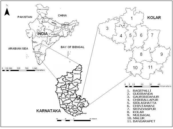
1.6 Study AreaBurgeoning population coupled with lack of holistic approaches in planning process has contributed to a major environmental impact in dry arid regions of Karnataka. Kolar district in Karnataka State, India was chosen for this study is located in the southern plain regions (semi arid agro-climatic zone) extending over an area of 8238.47 sq. km. between 77°21' to 78°35' E and 12°46' to 13°58' N (shown in Figure 1.1).
Figure 1. 1 : Study area Kolar district, Karnataka State, India
Kolar is divided into 11 taluks (or administrative boundaries / blocks / units) for administration purposes (Bagepalli, Bangarpet, Chikballapur, Chintamani, Gudibanda, Gauribidanur, Kolar, Malur, Mulbagal, Sidlaghatta, and Srinivaspur). The distribution of rainfall is during southwest and northeast monsoon seasons. The average population density of the district is about 2.09 persons / hectare.
The Kolar district forms part of northern extremity of the Bangalore plateau and since it lies off the coast, it does not enjoy the full benefit of northeast monsoon and being cut off by the high Western Ghats. The rainfall from the southwest monsoon is also prevented, depriving of both the monsoons and subjected to recurring drought. The rainfall is not only scanty but also erratic in nature. The district is devoid of significant perennial surface water resources. The ground water potential is also assessed to be limited. The terrain has a high runoff due to less vegetation cover contributing to erosion of top productive soil layer leading to poor crop yield. Out of about 280 thousand hectares of land under cultivation, 35% is under well and tank irrigation [39].