Accuracy Assessment

Image classification results in a raster file in which the individual raster elements are class labelled. As image classification is based on samples of the classes, the actual quality should be checked and quantified afterwards. This is usually done by a sampling approach in which a number of raster elements are selected and both the classification result and the true world class are computed. Comparison is done by creating an error matrix from which different accuracy measures can be calculated.

This chapter deals with the accuracy assessment of the LISS-3 MSS classified image (of spatial resolution 23.5 m) and MODIS classified image (of spatial resolution 250 m). The chapter is arranged into 3 sections. The first section (6.1) discusses the accuracy assessment of the LISS-3 supervised and unsupervised classification. MODIS classification accuracy assessment is shown in second section (6.2). Section 6.2 is further sub-divided into 2 sub sections. The first subsection (6.2.1) discusses the accuracy estimation of the MODIS hard classified maps. This assessment has been done at three levels – with the ground truth data collected from the field, at the administrative boundary level (Taluk level) and at the pixel level; by comparing on pixel by pixel basis with respect to LISS-3 classified map. The second subsection (6.2.2) shows the accuracy assessment of the soft classification at the administrative boundary level and at the pixel level, compared to LISS-3 classified image. The chapter concludes with a short discussion on the results of hard classification, soft classification and accuracy assessment (section 6.3).

Acronym used in this chapter:

•  MLC (LISS-3) – Maximum Likelihood classification on LISS-3 MSS.

•  K-Means (B1 to B7) – K- Means Clustering algorithm applied on MODIS Bands 1 to 7.

•  MLC (B1 to B7) – Maximum Likelihood classification on MODIS Bands 1 to 7

•  SAM (B1 to B7) – Spectral Angle Mapper applied on MODIS Bands 1 to 7.

•  NN (B1 to B7) – Neural Network applied on MODIS Bands 1 to 7.

•  DTA (B1 to B7) – Decision Tree Approach applied on MODIS Bands 1 to 7.

•  MLC (PCA) – Maximum Likelihood classification applied on PC 1 of MODIS 36 bands.

•  SAM (PCA) – Spectral Angle Mapper applied on PC 1 of MODIS 36 bands.

•  NN (PCA) - Neural Network applied on PC 1 of MODIS 36 bands.

•  DTA (PCA) – Decision Tree Approach applied on PC 1 of MODIS 36 bands.

•  MLC (MNF) – Maximum Likelihood classification on MNF 2 components of MODIS 36 bands.

•  SAM (MNF) – Spectral Angle Mapper applied on MNF 2 components of MODIS 36 bands.

•  NN (MNF) – Neural Network applied on MNF 2 components of MODIS 36 bands.

•  DTA (MNF) – Decision Tree Approach applied on MNF 2 components of MODIS 36 bands.

1 PC – Principal Components

2 MNF – Minimum Noise Fraction

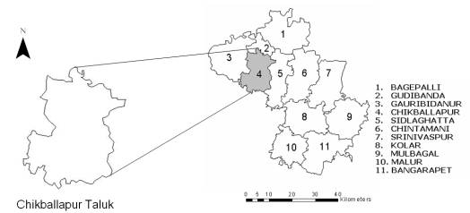
Accuracy assessment was done for Chikballapur administrative unit (taluk), where field data were collected on 5 th September and 25 th November 2005. Figure 6.1 shows overview of the Chikballapur taluk and its location in Kolar district. Table 6.1 gives the area of each taluk in hectares.

Figure 6. 1 : Chikballapur taluk in Kolar district where field data were collected.

The producer's and user's accuracy (as explained in chapter 4) corresponding to the various categories, and the overall accuracy were computed, along with the error matrices for supervised and unsupervised classified MSS data of LISS-3, which is summarised in table 6.2 and Annexure D (table 1 and 2). The LISS-3 supervised classification accuracy assessment gave a kappa (k) value of 0.95 indicating that an observed classification is in agreement to the order of 95 percent.

6.2 MODIS Classification Accuracy

6.2.1 Accuracy Assessment of hard classification for MODIS

User's (3) , Producer's ( 4 ) and Overall accuracy assessment of the MODIS classified maps (using hard classifier) was done for Chikballapur taluk with the ground truth data and the results are listed in Table 6.3, 6.4 and 6.5 respectively.

Table 6. 4 : User's Accuracy of classified MODIS Data of Chikballapur taluk.

(3) - It is a measure of commission error indicating the probability that a pixel classified into a given category actually

represents that category on the ground.

(4) - It indicates how well training set pixels of the given cover type are classified.

Table 6. 5 : Producer's Accuracy of classified MODIS Data of Chikballapur taluk.

From the overall accuracy assessment, NN on MNF and MLC classification on MODIS bands 1 to 7 performed better than the other techniques.

Comparison based on land cover class percentage area

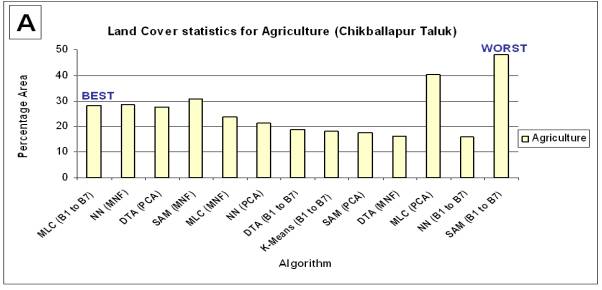
Accuracy Assessment of MODIS classified maps was also performed at two spatial scales – at the administrative boundary level (Taluk) and at the pixel level. Land cover statistics were computed for all taluks pertaining to each classification algorithm. Land cover percentage area versus various algorithms for Chikballapur is shown in table 6.6. Percentage area statistics for the six land cover classes were computed for all the taluks and were compared on the basis of the different algorithms (please see Annexure D, table 3 to table 13). Figure 6.2 shows the best (left) to worst (right) algorithms for land cover class mapping in Chikballapur taluk.

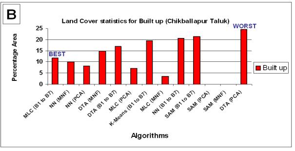
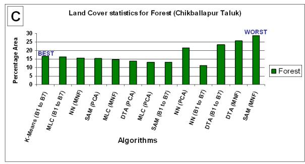
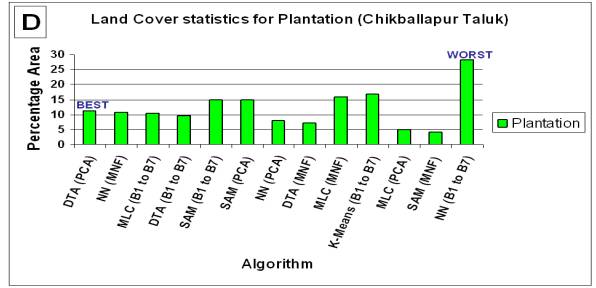
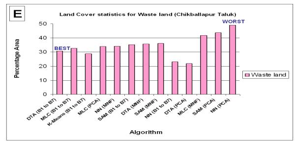
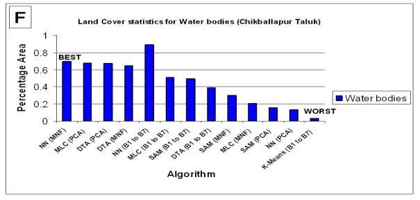
Figure 6. 2 : Best (left) to worst (right) classification algorithms for mapping land cover classes in Chikballapur taluk. LISS-3 MSS classified image is used for comparison.

The overall taluk wise percentage area for various algorithms shows that NN based classification on MODIS MNF is most comparable to LISS-3 classified image and is suitable for land cover classification at regional level. MLC on MODIS bands 1 to 7 also proved to be second best algorithm for classification.

Pixel to pixel analysis with LISS-3 MSS classified image

MODIS classified data were also compared with LISS-3 MSS classified data on a pixel by pixel basis for accuracy assessment of pure (homogenous) pixels. One pixel of MODIS spatially corresponds to 121 pixels (that is approximately equal to 258.5 m) of LISS-3. The error matrix was generated with user's accuracy, producer's accuracy and overall accuracy for the taluk and is listed in table 6.7, 6.8 and 6.9. This analysis also indicates that NN (MNF) classification technique is relatively better among 13 techniques.

Comparison on the basis of percentage area with LISS-3 MSS

Table 6.10 shows the land cover statistics for Chikballapur taluk obtained from the abundance maps generated using Linear Mixture Model (LMM), which is compared with LISS-3 classified map. All categories show comparable values of MODIS to LISS-3 except waterbodies that were overestimated in the area. For the land cover details of each taluk see Annexure D (table 14).

•  Accuracy Assessment based on Pixel Analysis

The taluk was divided into 16 quadrants of 5 min by 5 min (9 km by 9 km) gird and homogeneous (pure) pixels were verified in each grid. At the pixel level, a total of 51 parcels with respect to the six land cover classes were verified using handheld Magellan GPS in Chikballapur taluk and table 6.11 provides the validation results.

Waterbodies which constitute less than 1% of the total area in the district were misclassified and were wrongly estimated. Field verification showed that most of the pure pixels as well as few mixed pixels (for example agriculture with plantations/orchards, open forest class mixed with plantation and barren land mixed with urban class) were classified correctly.

6.3 Discussion

6.3.1 Hard Classification

Hard classification technique performs well with high spatial resolution as in the case with LISS-3 image when the actual ground cover is heterogeneous in nature. Good training site and ancillary data, along with minimum difference between the date of acquisition and date of ground truth collection further aids in achieving better classification result. MODIS classified image with coarse spatial resolution had many pixels that were misclassified as is clear from the Accuracy Assessment.

Further, within the land cover parameter, errors are generated when the classification algorithm selects the wrong class. With respect to a particular class, errors of omission occur when pixels of that class are assigned wrong labels; errors of commission occur when other pixels are wrongly assigned the label of the class considered. These errors occur when the signal of a pixel is ambiguous, perhaps as a result of spectral mixing, or when the signal is produced by a cover type that is not accounted for in the training process. These errors are a normal part of the classification process. They can be minimized, but not avoided entirely.

As additional argument it can be said that as pixel size increases, the chances of high accuracies in hard classifications being product of random assignment of values declines.

For Linear Mixture Modelling (LMM), the selection of the endmembers has an important effect. This is essential to properly identify different endmembers for MODIS since it proved to be highly relevant, as it is clear from the results that a high adjacency effect exists between contrasting features (forest and plantation, for example). When comparing LISS-3 MSS and MODIS, another important fact that can be attributed to LISS-3 is its spatial resolution (23.5), the reason for its superior results in the detection of the land cover class distribution and MODIS data having a coarse spatial resolution (250 m), where misclassification of the pixels are more likely.

The reason for the MODIS low accuracy can be the presence of another singularity: adjacency effects. The results suggest that this could be a limitation to the use of MODIS data in areas of high contrasting nature, as is the case of waterbodies, and raises concerns about its application especially on heavily fragmented or small isolated areas.

When unmixing an image to generate the abundance maps, from the presence of endmembers which do not mix in a linear fashion is a matter of concern. Errors in sensor operation and sensor noise can also add to the ones already mentioned. These errors take place when the selection of endmembers is wrong, for example when these do not correspond to pure pixels. The determination of endmember fractions for MODIS in the study area exhibits good behaviour in places where the endmembers are present, generally showing the capacity of estimating values within 20 % to 25 % of the actual values.

The Linear Spectral Unmixing (LSU) of MODIS on the other hand presents more errors which are avoidable. The overall values on the difference maps show only slight divergence, producing good estimates across the whole maps, except for the waterbodies endmembers. It suggest that the selection for this endmember could be improved, which is reasonable as this endmember shows high spectral variability (for example, clear water is different from turbid water or muddy water). When no more recognizable patterns are found and the RMSE is overall small, it can be deduced that a near perfect model has been reached.

The spectra of the different endmembers were modelled by linear equations. This introduces another form of quality assurance, as these equations can be inverted taking the endmember spectra to reconstruct the spectra of each pixel from the original image. Divergences between the original and

reconstructed image also give idea of the goodness of fit of the model, and give insights to which bands add more to the errors.

When assessing the accuracies of the image classifications, several things have to be kept in mind. The most important one is the way of data collection that served as input for the classification of the reference set.

Reference data include both ground truth data and other ancillary data. The time difference for the source data used in developing a reference dataset, the reference (field based) date and the MODIS and LISS-3 MSS acquisition dates impact both utility and accuracy of classified maps. Errors may have been introduced since the training data, the image and validation data are not temporally coincident with the sensor observations. Every possible measure was taken to minimize this effect, relating other ancillary data and vegetation presence information with the visual interpretation of the fused LISS-3 MSS (23.5 m) and IRS-1C/1D Panchromatic data (of spatial resolution 5.8 m) and having acquired information about that time from other sources. Nevertheless, even when counting with a high resolution image, which certainly helps to ameliorate the effects of the sampling, care has to be taken in the interpretation of the results, as the presence of bias is likely to happen. To summarize, it is not certain that the reference data in this case actually is representative of the entire classification.

Another source of bias that influences the conclusions that can be drawn from the classification is the quality in the co-registration of the images [134]. This is still a matter of consideration when working with MODIS data, as the quality of its georeferencing could mean a maximum of 10 to 15 % of error in the area of a pixel. Although care was taken in the geo-referencing process so as to minimize the RMSE error yet, small misregistration may be another significant source of error. Since each MODIS measurement is geolocated, this problem amounts to uncertainty in true geolocation. Therefore, although no accurate value can be given, it becomes evident that MODIS subpixel classification performance is definitely better, when mixed pixels are present.