|
FOREST ECOSYSTEM: GOODS AND SERVICES
|
| T.V. Ramachandra Subash Chandran M.D. Bharath Setturu Vinay S Bharath H. Aithal G. R. Rao |
| Energy & Wetlands Research Group, Centre for Ecological Sciences,
Indian Institute of Science, Bangalore, Karnataka, 560 012, India. E Mail: tvr@iisc.ac.in; Tel: 91-080-22933099, 2293 3503 extn 101, 107, 113 |
|
QUANTUM GIS (QGIS) – SPATIAL MAPPING TOOL
|
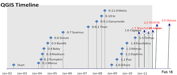
QGIS (http://qgis.org) is a Free and Open Source Geographic Information System for manipulating geographical data (vector, raster), statistical analysis. QGIS project was initiated on May of 2002 by Gary Sherman, established as a project on SourceForge. The first release was on July 19, 2002 and QGIS 3.0.0 'Girona' as the current version. QGIS is multiplatform GIS that runs on Windows, Unix, Linux platforms, macOS and Android. QGIS is a user-friendly GIS (https://www.qgis.org/en/site/forusers/download), providing common functions and features supports a number of raster and vector data formats. The plugin architecture provides access to new format support easily. QGIS is released under the GNU General Public License (GPL).
Installation:
- Download from URL https://www.qgis.org/en/site/index.html
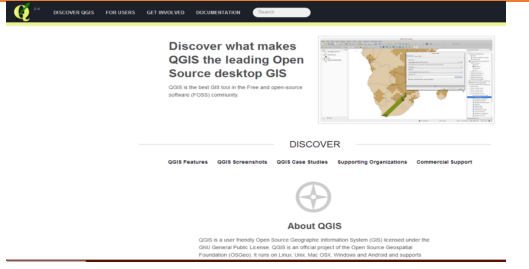
- QGIS main page will be opened as shown below.
- Download QGIS 2.18.17 LTR version
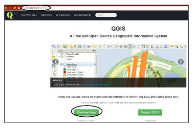
- Click on download now you will find the list of versions available.
- Download the latest stable (2.18.17 LTR) version.
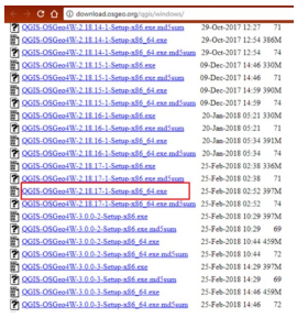
- Then it will be downloaded. Locate exe file in your computer.
- Double click on QGIS-OSGeo4W-2.18.17-1-Setup-x86_64.exe or QGIS-OSGeo4W-2.18.17-1-Setup-x86.exe.
- You will get QGIS 2.18 folder on desktop with following options QGIS Desktop; QGIS browser; QGIS Desktop with Grass support; QGIS Browser with Grass; Qt designer et.
- Click on QGIS Desktop icon.
- QGIS main window will be opened and looks as shown
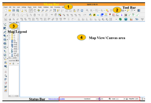
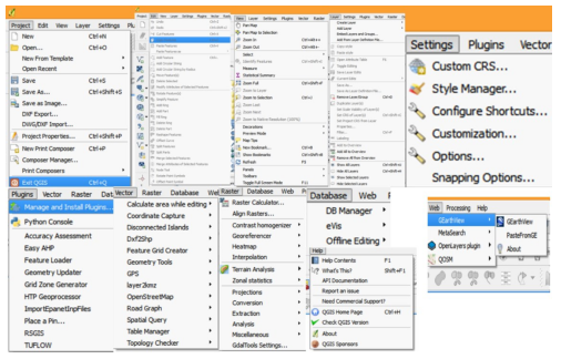
- The menu bar provides access to numerous QGIS features (Project option to Help)\

- The toolbars offer additional tools for interacting with the map. The toolbar provides access to most of the same functions as the menus, plus additional tools for interacting with the map. Hold your mouse over the item and a short description of the tool’s purpose will be displayed. Every toolbar can be moved around according to your needs.
- The map legend area sets the visibility
- QGIS - maps are displayed in map canvas area
- The map overview panel provides a full extent view of layers added
- The status bar shows the current position in map coordinates
Each session can be saved as a “Project”. The Print Composer helps in styling output images and saving thematic maps with layout and legends.
The following shows the different options available under each menu.
Working with Vector data
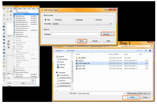
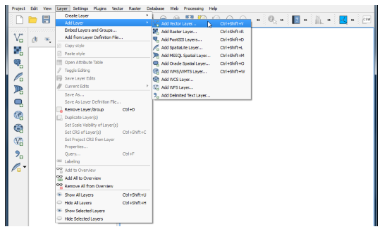
Vector files can be point, line, polygon forms store a description about any feature. QGIS support numerous vector data formats (Shape File, KML, Tab, MIF etc.). The most commonly used format is ESRI Shape File. To input vector data, click on Layer, then Add vector layer. Locate the vector file stored in your system, select “Filename.shp”, then vector feature will be loaded. You can change projection by right click properties or save as option to save a new file with you own projection. The global default CRS is EPSG:4326 - WGS 84 (proj=longlat +ellps=WGS84 +datum=WGS84 +no_defs). Options for global and project-wide CRS (Coordinate Reference System) for layers allows to define custom coordinate reference systems and supports on-the-fly (OTF) projection of vector and raster layers - Can display layers (with different CRS) and options for overlay. QGIS supports >2,700 known CRS. Definitions for each of these CRS are stored in a SQLite database that is installed with QGIS.
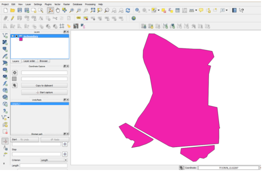
The selected vector file will be displayed as,
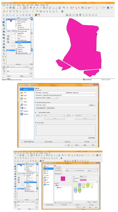
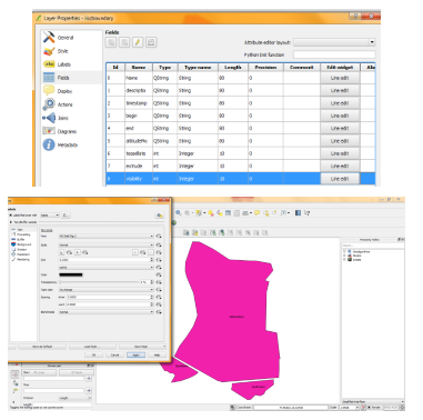
To improve performance then Right click on layer name select properties you will get options as, General, Styles, Labels, Attributes, Metadata, Actions, Joins, Diagram overlay.
- General will provide layer details such as where it is stored(path), projection etc.
- Labels help to label features (Description) of vector file.
- Styles allow you to change colours, patterns etc.
- Attributes will provide type such as Text, Integer, Real etc.
- Metadata description about layer and history.
- Joins allows you to link with another layer or text data.
Database ingest-querying:
Data ingestion is the process of obtaining, importing, and processing data. Process involves altering individual files by editing their content and fit into a larger document. Load vector file (Ex: IISc buildings shape file to see the Querying feature in QGIS).
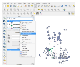
Right click on Layer name and click Open Attribute Table
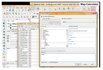
Attribute Table will be displayed with features already stored in the database. To compute area of buildings, click on Start editing (Pencil type icon) and click on Mapcalculator.
Add filed data type to be created to store data. Since Area is real value provide data type as Real with 2 precision width. Locate $Area under predefined Geometry functions. Click on it and press OK then Area will be computed stored in the Area column.
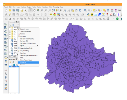
Creating Thematic Maps: Right click on BBMP Wards Vector file and see the attribute table byclicking Open Attribute Table. The layer has details such as Ward Name, Ward No, Population Male, Poulation Female, SC and ST population, Total Population etc. If we want to represent the Wards having population greater than 15000 and other categories in different colors, we use thematic map representation. Close Attribute Table. Right Click on Vector file name, click on Properties. Then Properties menu will show various options, click on Styling tool bar then by default Single Symbology will be shown click on that tab it will show the various options such as Single Symbology, Categorized, Graduated etc. Select on Graduated option. Then specify the column name to be used for Thematic map creation. Select Total Population column then click on Classify by default it will show 5 categories. If you want to reduce or increase you can specify. If you want your own ranges to be displayed click on the row1 and specify maximum break for each row. You can click on color symbol to change required color. You can also edit legend entry text to be shown as you wish. After all changes press Apply and click OK. Then the final output will be shown in Map Display.
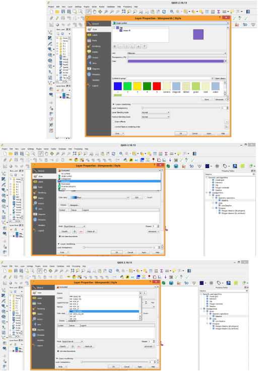
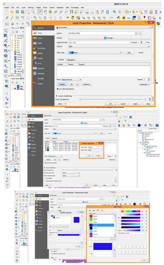
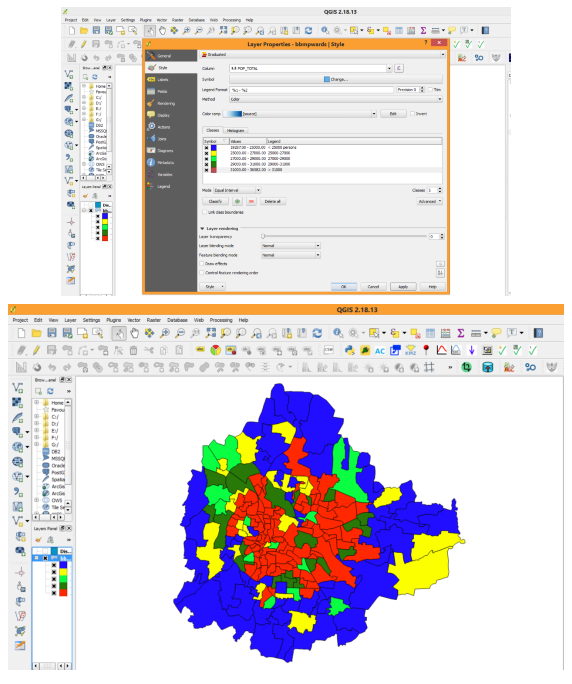
Use print composer option under Project section to save as JPG/PNG output file formats with Legend and Scale bar details.
Print composer has
● Apply map, legend, north arrow and text
● Using external programms (inkscape) for finetuning.
● Lots of paper formats supported; Separate DPI settings
● Logo inclusion, legend, labels, northarrow
● PNG/SVG/PDF support; Adjustable drawing scale
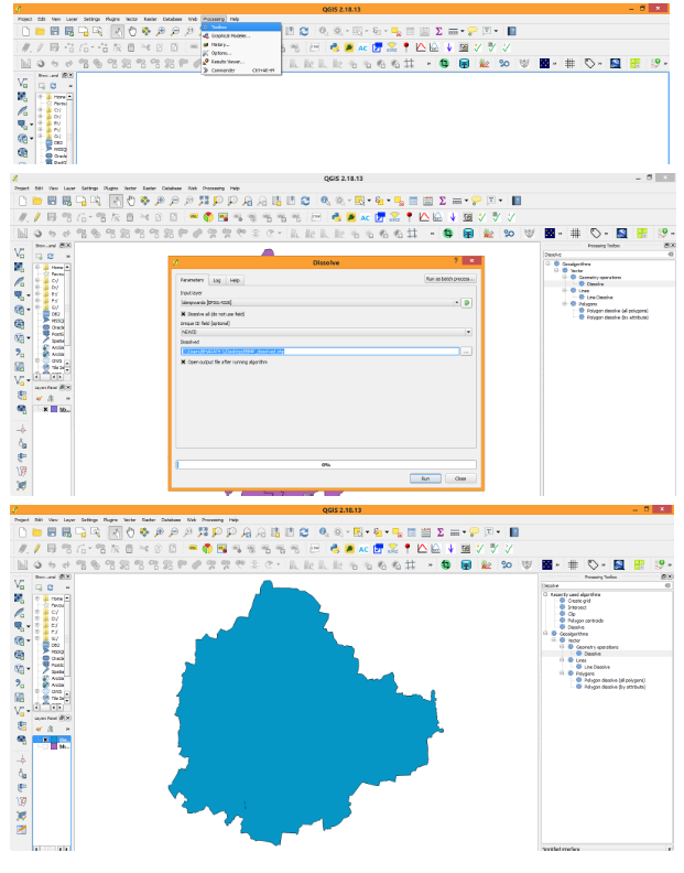
Dissolve: Dissolve tool is used to create a single vector boundary from a multiple vector files. For ex. we have provided BBMP ward boundaries file, to have a single BBMP boundary (Outer) then we will use Dissolve tool. For specifying a common field Right click on Layer name, Open Attribute Table. Click Toggle Editing then click on MapCalculator. Create a new field name as NewId, datatype as Integer. Just Type 1 in command operation section. Then a new field such as NewId has been created with all columns having Id as 1. Now stop Toggle Editing then save edits.
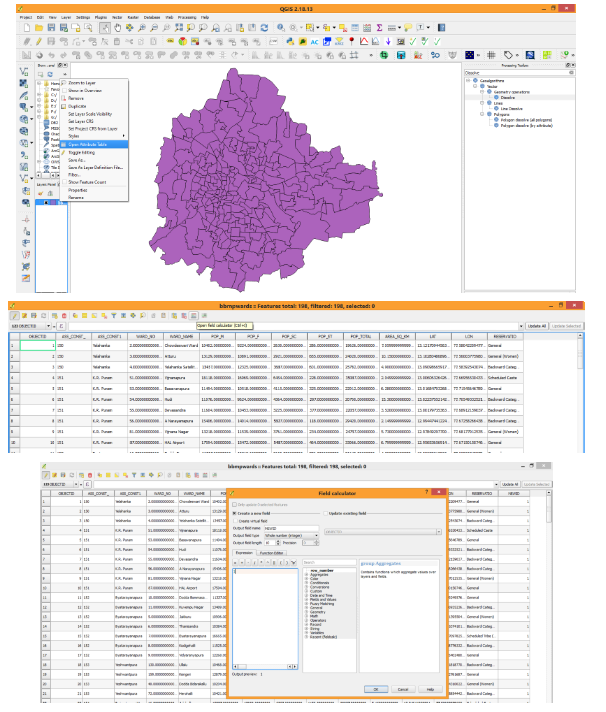
Click on Processing load tool box type “Dissolve”, then Dissolve tool will be shown under Vector Geometry operations section. Click on Dissolve tool then Dissolve tool GUI will be opened. It asks to load vector file input then indicate the filed to be dissolved. Click RUN to dissolve operation, then output will be shown.
Interpolation: Interpolation is used to create continuous surface from discrete points. It is a process of using points with known values to estimate values at other unknown points. A lot of real world phenomena are continuous - elevations, soils, temperatures, rainfall etc. If we wanted to model these, it is impossible to take measurements throughout the surface. Hence, the field measurements are taken at various points along the surface and the intermediate values are inferred by a process called ‘interpolation’. In QGIS, interpolation is achieved using the built-in Interpolation plugin. First import vector file or CSV file to be interpolated. If you are importing CSV then save it as Vector file.
Importing CSV file
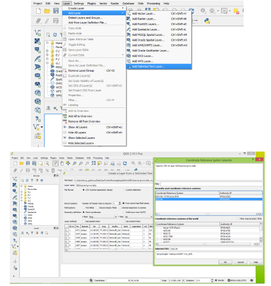
Then save as ESRI Shape file with “UTM Projection” by right click on layer name SaveAs Option.
Importing Vector file
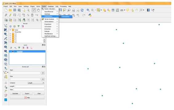
Click Raster option in Menu bar then click Interpolation and Interpolation. Provide Vector file name and column to be considered, raster cell size (30 m) and output file name.
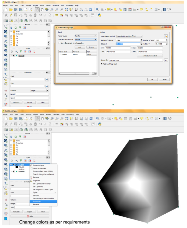
Run Zonal Statistic option available under Raster toolbar to compute ward wise Mean Rainfall.
Importing Google earth data:
- To load a vector file, click on Layer menu in menu bar select Add Vector Layer, a dialogue box will be displayed, which allows to traverse through the file system and load a kml file which you have created using Google earth or other formats of vector data.
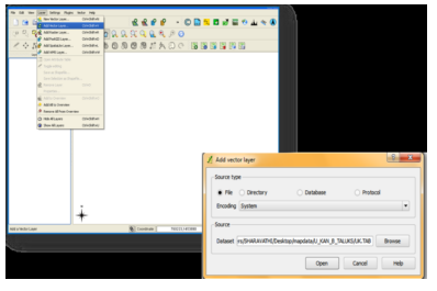
- The layer will be displayed in the map canvas area.
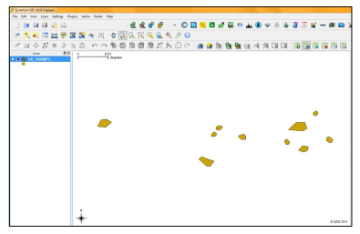
- Right click on the layer and select properties to check the attributes, colors etc.
- QGIS supports a number of Symbology renderers to control how vector features are displayed
- Labels tab allows to enable labelling features and control a number of options related to fonts, placement, style, alignment and buffering.
- Right click on the layer click save as option to create a shape file and specify co-ordinate reference system to be saved (CRS), then specify output file name.
- Import the shape file and continue to work with it. So you can edit the features and compute the area etc.
Working with Raster data:
Geo referencing
- Geo-referencing is the process of assigning real earth coordinates to the digitised maps, so it can be viewed, queried, and analysed with other geographic data.
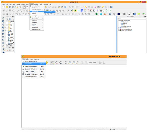
- To start geo referencing an unreferenced raster, we must load it by clicking Georeferencer option in the Raster menu bar and click on Georeferencer.
- The Georeferencer window will be opened click on File menu and click Add raster layer. The raster will show up in the main working area of the dialog. Once the raster layer is loaded, we can start to enter reference points.
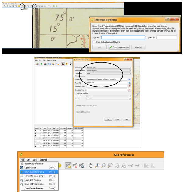
- Using the Add Point button (Edità Add points), you can add points to the main working area and enter their coordinates. Click on a point in the raster image which you want to assign co-ordinates and enter the X and Y coordinates manually. With the move button option, you can move the GCPs (Ground control points) on map, if they are at the wrong place. X should be longitude and Y should be latitude.
- Continue entering points. You should have at least 4 points and the more coordinates you can provide, the better the result will be. There are additional tools on the plugin dialog to zoom and pan the working area in order to locate a relevant set of GCP points.
- After entering GCP’s click on Settings option in Georeferencing menu bar select Transformation Settings option. A drop box will be displayed and select options as shown in the below image. Specify output file name and transformation parameters and projection system then click OK.
- Click on File menu and Select Start Georeferncing option. The Georefrencing will be started.
Digitising features (vector data) from Raster data:
Digitising features (water bodies) from Topo map:
- Open the raster file you have geo referenced by clicking Layerà Add raster layer option.
- The raster layer window will be open and load the saved layer. It will be displayed on Map canvas.
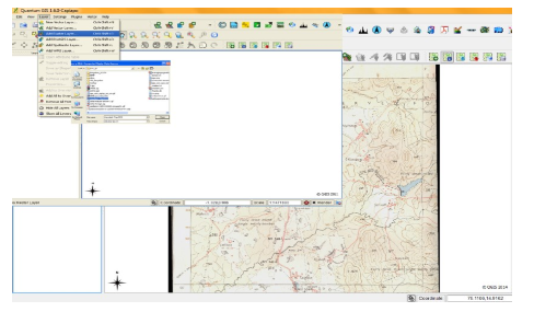
- To digitise the water bodies select Layer menu and click Newàcreate new shape file layer option. Then new shape file layer drop box will open with options.
- Select polygon option and provide the attributes for it and save the file with a name. The saved new shape file will be loaded for creation of features.
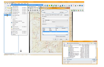
- Attributes are entered as features to be created.
- Zoom to the feature you want to digitize by using zoom options. Right click on the vector layer you have created and select Toggle editing (pencil like symbol) option. Then tool bar will be highlighted. Click on capture polygon icon and start digitizing the water body.
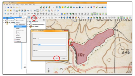
- Enter the attributes and press ok. After digitisation click save layer option to save the modifications you made.
- To compute area of the polygon right click on the layer you digitised and click open attribute table and select field calculator select area option to compute area.
- The area will be shown in degrees. Convert it to Hectares by adding new column and provide the name for new column. Then select field calculator select the new column to be updated.
- Type the formula as AREA*110*110*10000 for getting in terms of Ha.
Help from QGIS:
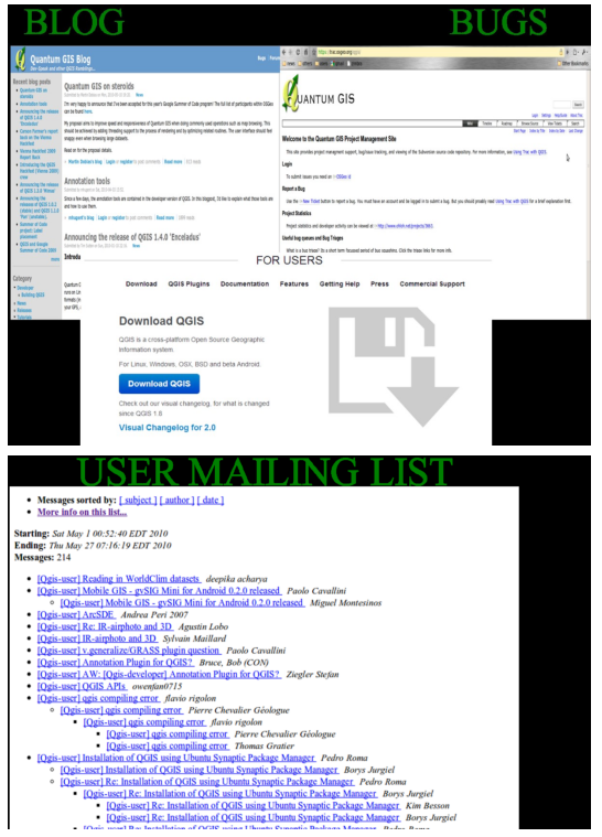
QGIS has active community support, update and upgrades
http://wgbis.ces.iisc.ac.in/biodiversity/
http://www.qgis.org/en/site/forusers/index.html#
http://www.qgis.org/en/docs/index.html
http://wgbis.ces.iisc.ac.in/grass/
http://wgbis.ces.iisc.ac.in/foss/
http://wgbis.ces.iisc.ac.in/energy/water/paper/researchpaper2.html#f
http://wgbis.ces.iisc.ac.in/biodiversity/pubs/ETR/index.htm
