Basic Data Models

GIS depicts the real world through models involving geometry, attributes, relations, and data quality. In this chapter, the realization of models is described, with the emphasis on geometric spatial information, attributes, and relations.   Spatial information is presented in two ways: as vector data in the form of points, lines, and areas (polygons); or as grid data in the form of uniform, systematically organized cells. Geometric presentations are commonly called digital maps. Strictly speaking, a digital map would be peculiar because it would comprise only numbers (digits). By their very nature, maps are analog, whether they are drawn by hand or machine, or whether they appear on paper or displayed on a screen. Technically speaking, GIS does not produce digital maps—it produces analog maps from digital map data. Nonetheless, the term digital map is now widely used that the distinction is well understood.

Vector Data Model: The basis of the vector model is the assumption that the real world can be divided into clearly defined elements where each element consists an identifiable object with its own geometry of points, lines, or areas (Figure 4.1). In principle, every point on a map and every point in the terrain it represents is uniquely located using two or three numbers in a coordinate system, such as in the northing, easting, and elevation Cartesian coordinate system. On maps, coordinate systems are commonly displayed in grids with location numbers along the map edges. On the ground, coordinate systems are imaginary, yet marked out by survey control stations. Data usually may be transformed from one coordinate system to another.  With few exceptions, digital representations of spatial information in a vector model are based on individual points and their coordinates. The exceptions include cases where lines or parts of lines (e.g., those representing roads or property boundaries) may be described by mathematical functions, such as those for circles or parabolas. In these cases, GIS data include equation parameters: for example, the radii of the circles used to describe parts of lines. Together with the coordinate data, instructions are entered as to which points in a line are unconnected and which are connected. These instructions can subsequently be used to create lines and polygons and to trigger “pen up” and “pen down” functions in drawing.

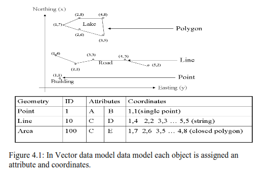
Coordinate systems are usually structured so that surveys along an axis register objects in a scale of 1:1; that is, 1 m along the axis corresponds to 1 m along the ground. In principle, the type of measuring method applied, while the required degree of precision will naturally influence the amount of work required to gather the data, decides the degree of accuracy of measurements along an axis. Mathematically, a vector is a straight line, having both magnitude and direction. Therefore, a straight line between two data coordinate points on a digital map is a vector—hence the concept of vector data used in GIS and the designation of vector-based systems. In a vector model, points, lines, and areas (polygons) are the homogeneous and discrete units that carry information. As discussed above, these three types of object may be represented graphically using coordinate data. However, as we shall see, the objects may also carry attributes that can be digitised, and all digital information can be stored.

 

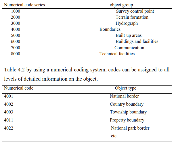
Coding digital map for map production: Anyone familiar with maps knows that map data are traditionally coded. Roads, contour lines, property boundaries, and other data indicated by lines are usually shown in lines of various widths and colours. Symbols designate the locations of churches, airports, another buildings and facilities. In other words, coordinates and coding information identify all objects shown on map. Not surprisingly, than, the digital data used to produce maps are also coded,  usually by the assignment of numerical codes used throughout the production process—from the initial data to computer manipulation and on to the drawing of the final map. Each numerical code series contains specific codes assigned to objects in the group. For example, the codes for boundaries may be illustrated in table 4.1 and 4.2

Table 4.1 digital map data often use numerical coding, in the form of different numerical series, to identify object groups.

Digital data for map production comprise sequences of integers, such as
-53144011123456789123406780-53144011123336788123306700

Use of the format permits the numerical sequence to be divided into groups and read
-5/ 314/ 4011/ 12345/ 6789/ 12340/ 6780
-5/ 315/ 4011/ 12333/ 6788/ 12330/ 6700

The figures designations are as follows:

Figure               Designates

-5                  Start of a continuous sequence of data (i.e., if there are several                                                            coordinates, they are to be connected in a line: pen down)

314                 Serial number of data sequence (such as of a unique line)

4011              Property boundary (such as might produce a final line width of 0.3 mm)

12345             First easting coordinate

6789                First northing coordinate (pen moves to next coordinate set).

12340             Last easting coordinate

6780               Last northing coordinate

 

-5                End of data sequence, start of next sequence (pen up—moved and set  down for a sequence of new coordinate, etc.)

 

In thematic coding, which may be compared to the overlay separation of conventional map production, data are divided into single-topic groups, such as all property boundaries. Information on symbol types, line widths, colours, and so on, may be appended to each thematic code, and various combinations of themes may be drawn. Data may be presented jointly in this way only if all objects are registered, using a common coordinate system.

Coding digital data for GIS

Point objects may easily be realized in a database because a given number of attributes and coordinates is associated with each point (Figure 4.1). Line and polygon objects are more difficult to realize in a database because of the variation in the number of points composing them. A line or a polygon may comprise two points or 2000 or more points, depending on the extent of the line and the complexity of the area, which is delineated by a boundary line that begins and ends at the same point. Object spatial information and object attributes are often stored in different databases to ease the manipulation of lines and areas, but in some systems they are stored together. As pivotal attributes are often available in existing computer memory files, dividing the databases conserves memory by precluding duplicate storage of the same data. The separate storage of attribute and spatial information data requires that all objects in the attribute tables be associated with the corresponding spatial information. This association is achieved by inserting spatially stable and relevant attribute data or codes form the attribute table into the special information, or vice-versa. In other words, identical objects have the same identities in both databases. The identity (ID) codes used to label and connect spatial information and attribute table data are most often numerical, but may be alphanumerical. Typical identity codes include building numbers, property numbers and addresses. If the data are ordered in a manuscript map, each object may be assigned a serial number used in both the spatial information and the attribute databases. Polygons for vegetation mapping can, for example, be numbered from 1 onward, while pipes, manholes, and so on, are usually numbered according to an administrative system. ID codes allow differentiation between objects, whereas theme codes allow differentiation between different groups of objects. In theory, identity codes and thematic codes are both attributive data. However, they are very closely tied to geometry and are therefore often treated as such, as described above.

Table 4.3: typical section of digital map data with relevant code list

I.D.	Thematic code	X-coordinates (degree)	Y-coordinate (degree)
11 34 - 122	30 30 40 40 - - 20	74.562323 74.253686 74.567815 75.646433 - - 75.894625	14.035566 14.235891 14.256874 14.872566 - - 15.564615

     Spatially defined objects without attributes need no identifiers, but they are required for all objects that are listed in attribute tables, and manipulated spatially. Identifiers are normally entered together with the relevant data, but they may also be entered later, using an interactive human—machine process such as keying in identifiers for objects pointed out on the screen.
Some systems tie a polygon’s ID code to a characteristic point in the polygon, known as the label point. Label points may be computed or identified interactively on the screen, and codes may be entered manually for the relevant polygons. The attribute values of the polygon are then linked to this label point. Today, systems are available which treat polygons as independent objects. Typical digital geometric data for GIS are illustrated in table 4.3.
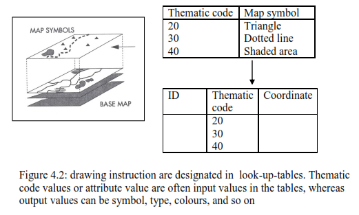
Plotting may be controlled by appending drawing instructions to the thematic code, to the individual identifiers, or to other object attributive values. In a finished map, tabular data appear on a foreground amp against the background of a base map derived from the remaining map data. Look-up tables are usually used to translate tabular data map symbols (Figure 4.2).

 

 

Spaghetti model

Digital map data comprise lines of contiguous numerals pertaining to spatially referenced points. Spaghetti data are a collection of points and line segments with no real connection (Figure 4.3). What appears as a long, continuous line on the map or in the terrain may consist of several line segments which are to be found in odd places in the data file. There are no specific points that designate where lines might cross, nor are there any details of logical relationships between objects. Polygons are represented by their circumscribing boundaries, as a string of coordinates so that common boundaries between adjacent polygons are registered twice (often with slightly differing coordinated). The lines of data are unlinked and together are a confusion of crossings.

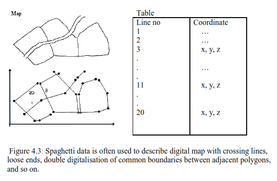
Unlinked (spaghetti) data usually include data derived either from the manual digitising of maps or from digital photogrammetric registration. Consequently, spaghetti data are often viewed as raw digital data. These data are amenable to graphic presentation— the delineation of borders, for example—even though they may not form completely closed polygons. Otherwise, their usefulness in GIS applications is severely limited.
One drawback is that both data storage and data searches are sequential. Hence search times are often unduly long for such routine operations as finding commonality between two polygons, determining line intersection points, or identifying points within a given geographical area. Other operations vital in GIS, such as overlaying and network analysis, are intractable. Furthermore, unlinked data require an inordinate amount of storage memory because all polygons are stored as independent coordinate sequences, which means that all lines common to two neighbouring polygons are stored twice. The typical memory required for unlinked data is illustrated in table 4.4

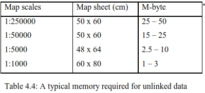
Topology model

Topology is the branch of mathematics that deals with geometric properties which remain invariable under certain transformations, such as stretching or bending. The topology model is one in which the connections and relationships between objects are described independent of their coordinates; their topology remains fixed  as geometry is stretched and bent. Hence the topology model overcomes the major weakness of the spaghetti model, which lacks the relationships requisite to many GIS manipulations and presentations.

The topology model is based on mathematical graph theory and employs nodes and links. A node can be a point where two lines intersect, an endpoint on a line, or a given point on a line. For example, I a road network the intersection of two roads, the end of a cul-de-sac, or a tunnel adit may generate a node. A link is a segment of a line between two nodes. Links connect to each other only at nodes. A closed polygon consisting of alternating nodes and links forms an area. Single points can be looked upon as a degenerate node and as a link with zero length (Laurini and Thompson 1992). Theme codes should be taken into consideration when creating nodes to ensure that they are created only between relevant themes (e.g., at the junction between a national highway and a county road, not between roads and property boundaries).

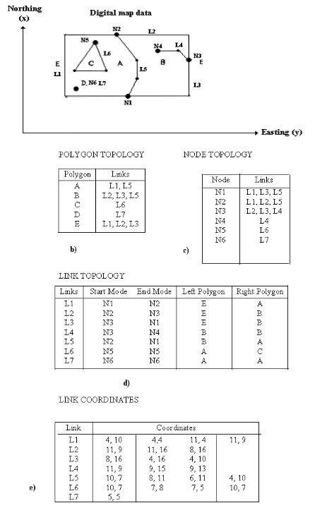
Figure 4.4: Topology model: a)digital map data can be  represented by nodes and links. b) a polygon table; c) a node topology table, and d) a link topology table. e) geographical coordinates

Unique identities are assigned to all links, nodes, and polygons, and attribute data describing connections are associated with all identities. Topology can therefore be described in three tables (figure 4.4):The polygon topology table lists the links comprising all polygons, each of which is identified by a number.

1. The node topology table lists the links that meet at each node.

2. the link topology table lists the nodes on which each link terminates and the polygons on the right and left of each link, with right and left defined in the direction from a designated start node to a finish code. The system creates these tables automatically.

A table with point coordinates to the links ties these features to the real world and permits computations of distances, areas, intersections, and other numerical parameters. The geometry of the objects is stored in its own subordinate table (see Figure 4.4). Numerous spatial analyses may then be performed, including:

• Overlaying

• Network analyses

• Contiguity analyses

• Connectivity analyses

 

Topological attribute data may be used directly in contiguity analyses and other manipulations with no intervening, time-consuming geometric operations.

       Once the topology has been created, a map can be plotted with solid colours. This is not possible with spaghetti data. Thematic layers of topological data can also be used to steer the plotting sequence. The sequence influences what becomes visible on the map. For example, a green area superimposed on a white house will render the house invisible on the map (unless the house creates a window in the area).

        Topology requires that all lines should be connected, all polygons closed, and all loose ends removed. Even gaps as small as 0.001 mm may be excessive, so errors should be removed either prior to or during the compilation of topological tables.

        A function known as snap can also be used in digitisation. Using the snap function with a defined tolerance of, say, 1 mm, a search can be carried out around the end of a line or around an existing point which is assumed to have the same coordinates as the last point registered. When this point is found, the two points will be snapped together to form a common node, thereby closing the polygon. The same procedure can be carried out automatically on existing data. A node can also be created in existing data by calculating the point of intersection between lines. Meaningless loose ends can be removed by testing with a  given minimum length.
Topological information permits automatic verification of data consistency to detect such errors as the incomplete closing of polygons during the encoding process. The graph theory contains formulas for the calculation of such data errors. There has to be a fixed relationship between the number of nodes, lines, and polygons in one data set. A run-through of the data in positive and negative directions will produce the same result.

         The topological model has a few drawbacks. The computational time required to identify all nodes may be relatively long. Uncertainties and errors may easily arise in connection with the closing of polygons and formation of nodes in complex networks (such as in road interchanges). Operators must solve such problems. When raw data are entered and existing data updated, new nodes must be computed and the topology tables brought up to date.

          Topological data may require a longer plotting time than spaghetti data because of the separation of lines into nodes and links. However, the overall advantages of the topology model over the spaghetti model make it the prime choice in most GISs. Today, efficient software and faster computers enable topology to be established on-the-fly; thus the disadvantages of topological data as compared to spaghetti data have become less important.

          Here it suffices to say that usually. Map data are not stored in a contiguous unit, but rather, divided into lesser units that are stored according to a selected structure. This structure may be completely invisible to the user, but its effects, such as rapid screen presentation of a magnified portion of a map, are readily observable.

Data Compression

The amount of computer resources (memory and storage space) needed can be reduced by using data compression techniques. Most of these automatic techniques are based on removing points from continuous lines (contour lines, etc.). Good data compression techniques, therefore are those that preserve the highest possible degree of geometric accuracy. The most basic technique involves the elimination of repetitive characters: for example, the first character of all coordinates along a particular axis. The repetitive character needs to be entered only once; subsequently, it may be added to each set of coordinates. The particular technique has no effect on the geometry.

There are other automatic methods of removing points. One simple means is to keep only every nth point on the line. The lower the value of n, the greater the number of points that will be removed. This method does not take into account geometric accuracy; however, this can be compensated for by testing the curvature of the line. One method is to draw a straight line between the first and last points on a curved stretch of line and to calculate the orthogonal distance from each point on the curve line below the straight one. Points that are closer than a given distance from the straight line will be removed. The endpoint of the straight line is then moved to the point with the greatest distance and the same procedure for removing points is repeated. This continues until all the relevant points are removed. This method is known as the Douglas-Peucker algorithm.

 Points of little or no value in describing a line may be eliminated by moving a corridor step by step along a line and deleting points that are closer to the neighbouring point than a given value or where the vectors create an angle that is smaller than the given value. Contours and other lines can also be replaced with mathematical functions, such as straight lines, parabolas, and polynomials. A spline function comprises segments of polynomials joined smoothly at a finite number of points so as to approximate a line. A spline function can involve several polynomials to build a complex shape. It has been reported that a spline function representing nautical chart data has reduced data volume by 95%.

The amount of memory required to store a given amount of data often depends on the format in which data are entered. Some formats contain more administrative routines than others, some have vacant space. Thus, the gross volumes stored are frequently related to format.

Storing vector data

The manner in which digital map data are stored in a record is determined by a format, a set of instructions specifying how data are arranged in fields. The latter are groups of characters or words, which, in turn, are treated as units of data. The format stipulates how the computer will read data into the fields: total number of fields specified, number of characters permissible in each field, number of spaces between fields, which fields are numeric and which are text, and so on.

He information content of the data is designated not in the format but ancillary to it, for example, in a heading. Typical specifications for information content might include field assignments, such as the point number in the first field, the thematic code in the second, easting in the third, northing in the fourth, and elevation in the fifth. The meanings of the numeric codes used must also be given. The spaghetti data are stored in simple file structure and in order in which the data have been registered.
Users of conventional maps know the frustrations of extracting information from maps produced by various agencies using differing map sheet series, varying scales and coordinate systems, and frequently, different symbols for the same themes. Moreover, the graphic version of Murphy’s law dictates that the necessary information is all too often located in the corners where four adjoining map sheets meet.

Database storage of cartographic data can overcome these problems because it involves standardization of data through common reference systems and uniform formats. Cartographic data from various sources can, with few limitations, be combined. The results are then independent of map sheet series and scales.

Standardized storage makes the presentation of data compiled from dissimilar sources much easier. For example, uniform storage formats permit the combination of telecommunications administration network data with property survey data, or of geological information from 1: 50,000 scale maps with vegetation data from 1: 20,000 scale maps.

Digital map data are stored in databases, the computerised equivalent of conventional file drawers and cabinets. Although data entries in a database can be updated far more rapidly than data printed on map sheets on file, the information is found more quickly from map sheets than by searching in a database. This is because a single map sheet contains an enormous amount of information, usually equivalent to 100,000 or more sets of coordinates. A sequential computer search of 100,000 items in a database is slow even for the most powerful computers in comparison with a quick visual scan of a map sheet. Therefore, “smart” programs known as database management systems (DBMSs) have been compiled to maintain, access, and manipulate databases. The various DBMSs differ primarily in the ways in which data are organized. Their selection and use are vital in GIS applications because they determine the speed and flexibility with which data may be accessed.

It is usual to split topological data into different thematic layers to simplify storage and to improve access to data. This division is done so that no overlap occurs between polygons within each thematic layer. For example, property boundaries are stored in one layer while other data overlapping the property, such as roads, buildings, and vegetation boundaries, are stored in another. The disadvantage of this system is that common lines between objects (e.g., roads and properties) that are stored in different layers have to be removed several times. This problem can be avoided by using object-based storage.

Comments on spaghetti and topology models
When digitising lines such as those on land-use maps, the borders of surfaces are digitised both as spaghetti data and as separate objects. When creating topology, this model is converted to a layer model. The discussion of spaghetti and topology is very much based on the assumption that a class of area entities is always a tiling of the plane in which every point lies in exactly one polygon.  However, the problems related to spaghetti and topology have changed somewhat during recent years with the advent of new GIS software which treats polygons as independent objects that may overlap and need not fill the plane, and with systems permitting shapes. Many of the traditional arguments for area coverage/ layer model and use of topology are based on the assumption of needing to avoid computation. New and more powerful computers eliminate the need for reduction in calculation time. Today, topology can easily be built on-the-fly.

Raster data models

Raster data are applied in at least four ways:

1. Modelling describing the real world

2. Digital maps scans of exiting maps

3. Compiling digital satellite and image data

4. Automatic drawing by raster output units

In the first example, raster data are associated with selected data models of real world: in the second and third, with compilation method, and in the fourth, with presentation methods. The respective computer manipulation may be entered in a raster model. 

Raster models

Raster model represents reality through selected surface arranged in a regular pattern. Reality is thus generalised in terms of uniform, regular cells, which are usually rectangular or square but may be triangular or hexagonal. The raster model is in many ways a mathematical model, as represented by the regular cell pattern. Because square or rectangles are often used and a pictorial view of them resembles a classic grid of squares, it is sometimes called the grid model. Geometric resolution of the model depends on the size of the cell.  With in each cell the terrain is assumed to be flat.  

The rectangular raster cells, usually of uniform size throughout a model, affect the final drawing in two ways. First, lines that are continuous and smooth in a vector model will become jagged, with the jag size corresponding to the cell size. Second, resolution is constant: region with few variation are as detailed as those with major variations, and vice versa. 

The cells of a model are given in a sequence determined by a hierarchy of rows and column in a matrix, with numbering usually starting from the upper left corner (figure 4.2). The geometric location of cell, and hence of the object it represents, is stated in terms of its directional and column number. This identification corresponds to the directional coordinates of the vector model. The cells are often called pixel. A pixel is the smallest element of an image that can be processed and displayed individually. The raster techniques used in GIS are sibling of the raster long used to facilitate the manipulation and display of the information and consequently are suited to computerised technique.  

Realizing the raster model

Raster models are created by assigning real-world values to pixels (Figure 4.5). The assigned values comprise the attributes of the objects that the cells represent—and because the cells themselves are in a raster, only the assigned values are stored. Values, usually alphanumeric, should be assigned to all the pixels in a raster. Otherwise, there is little purpose in drawing empty rows and columns in a raster.

     Consider a grid of cells superimposed on the ground or on a map. Assigning the values/ codes of the underlying objects/ features to the cells creates the model. The approach is comprehensive because everything covered by the raster is included in the model. Draping a ground surface in this way regards the ground or map as a plane  surface.

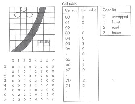
Figure 4.5: a line and column number define the cell’s position in the raster data. The data are then stored in a table giving the number and attribute value of each cell

 

  Some GISs can manipulate both numerical values and text values (such as types of vegetation). Hence cell values may represent numerous phenomena, including:

• Physical variables, such as precipitation and topography, respectively, with amounts and elevations assigned to the cells

• Administrative regions, with codes for urban districts, statistical units, and so on

• Land use, with cell values from a classification system

• References to tables of information pertaining to the area(s) the cells cover, such as references to attribute tables

• Distances from a given object

• Emitted and/or reflected energy as a function of wavelength—satellite data

 

     A single cell may be assigned only one value, so dissimilar objects and their values must be assigned to different raster layers, each of which deals with one thematic topic (figure 4.6). Hence in raster models as in vector models, there are thematic layers for topography, water supply systems, land use, and soil type. However, because of the differences in the way attribute information is manipulated, raster models usually have more layers than those in vector models. In a vector model, attributes are assigned directly to objects. For instance, pH value might be assigned directly to the object “lake”. In a raster model, the equivalent assignment requires one thematic layer for the lake, in which cells are assigned to the lake in question, and a second thematic layer for the cells carrying the pH values. Raster databases may, therefore, contain hundreds of thematic layers. 
In practice, a single cell may cover parts of two or more objects or values. Normally, the value assigned is that of the object taking up the greater part of the cell’s area, or of the object at the middle of the cell, or that of an average computed for the whole of the cells. Cell locations, defined in terms of rows and columns, may be transformed to rectangular ground coordinates, for example, by assigning ground coordinates to the centre of the upper left cell of a raster (cell 0, 0). If the raster is to be oriented north- south, the columns are aligned along the northing axis and the rows along the existing axis. The coordinates of all cell corners and centres can then be computed using the known cell shapes and sizes.
Object relations, which in the vector model are described by topology, are only partly inherent in the raster structure. When the row and column numbers of a cell are known, the locations of neighbouring cells can easily be calculated. In the same way, cells contained ii a given polygon may be located simply searching with a stipulated value. It is much more difficult, however, to identify all the cells located on the border between two polygons. Polygon areas are determined merely by adding up constituent cells. Some operations, though, are more cumbersome. An example, of this is computation of a polygon’s perimeter length, which requires a search for, and identification of, all the cells along the polygon’s border.

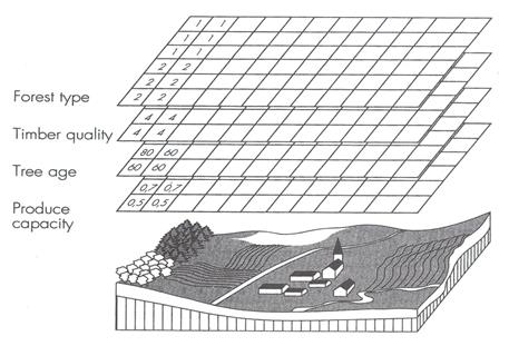
Figure 4.6: only one attribute value may be assigned to each cell. Objects that have several attributes are therefore represented with a number of raster layers, one for each attribute

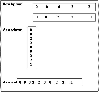
Figure 4.7: typical cell input. Raster data may be stored in the database as series of rows, a series of columns, or a continuous line.

 

 

Figure 4.7: typical cell input. Raster data may be stored in the database as series of rows, a series of columns, or a continuous line.
Overviews of phenomena in a given area are obtained from a raster model quickly and easily b searching all the thematic layers for cells with the same row and column numbers. The relevant overlay analysis is described later. Raster data are normally stored as a matrix, as described above. However, they can also be stored in tabular form, where each individual cell in a raster forms a line in the table (see Figure 4.7)

Coding raster data

Numerical codes and, in some systems, text codes may be assigned to cells. Cell values are entered from word processing files, databases, or other sources in the same sequence as they are registered (Figure 4.7). The way in which the figures are read is dictated by format. For instance, it is essential to know the number of columns per row. Raster data may be available from a variety of dissimilar sources, ranging from satellite data and data entered manually to digital elevation data. Their collocation requires that cells from differing sources and thematic layers correspond with each other. In other words, cells having the same row and column numbers must refer to the same ground area. Various computations may be necessary to accommodate any differences in cell shape and size.  Cells may contain values referenced to attribute tables. The cells of a thematic layer may be coded so that their values correspond to identities in a given attribute table. Attribute data or tabular data may be coded independently; irrespective of whether the geometry is represented using vector data or raster data.

Compression of raster data

It the cell values of a raster model are entered in fixed matrices with rows and columns identical to those of the registered data, only the cell values need to be stored; row and column numbers need not. Even when only the cell values are stored, the volumes of data can easily become unwieldy. Typical operations may involve 200 thematic layers, each containing 5000 cells. The total number of cell values stored is thus 200 x 5000 =1 million. A land sat satellite raster image contains about 7 million pixels, a Landsat TM image about 35 million pixels.

     Various devices may be employed to reduce data volume and, consequently, storage memory requirements. Cells of the same value are often neighbours because they pertain to the same soil type, the same population density of an area, or other similar parameters. Thus cells of the same value in a row may be compacted by stating the value and their total. This type of compacting, called run-length encoding. Further compacting may be achieved by applying the same process recursively to subsequent lines.