METHODOLOGY

The preliminary method adopted was to collect secondary data regarding the vegetation, forest cover, topography, species diversity, landuse in the past etc. of the study area, from governmental organisations such as forest department, forest research institutes, as well as non-governmental institutes such as French Institute, Pondicherry. Data was also obtained from reviewing certain literature works, which were of significant importance to this study. Apart from these, field investigations were undertaken in order to ascertain the spectral signatures in the remotely sensed data with ground condition – type of patch, type of vegetation, etc. After collecting the essential information required for this study, the digital analysis of these data was carried out. The methodology adopted for carrying out this analysis could be categorised into 4 steps as follows:

1. Digitization
2. Ground truth data
3. Remote sensing data
4. Digital Image Processing
5. Data analyses, data integration

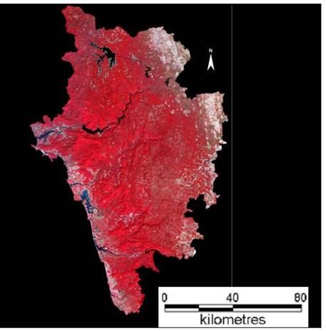
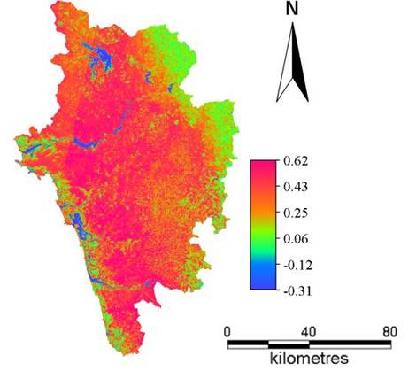
DIGITIZATION: Survey of India (SOI) topographical maps of scale 1:50,000 and 1:2,50,000, covering all taluks of Uttara Kannada district depicting taluk boundaries, road and rail network, and drainage pattern (Figure 2) were digitized.  The district boundary was digitized using toposheets 48 J, 48 I, 48 M, and 48 N each of scale 1:2,50,000.  The taluk boundaries, road and rail network, and the drainage network were digitized from toposheets of scale 1:50,000. The RMS errors for digitization were checked and found to be within the acceptable limits for the scales of maps used.  The lat/long coordinate system was used for digitization. Vegetation map of South India (Figure 5) of scale 1:2,50,000 was digitized using Vegetation map developed by French Institute (1984). This helps in temporal analyses to find out the changes in vegetation during the last twenty years.

These digitized images (major road network and drainage network) were used to georegister and also to implement geo correction of the satellite imageries.  Vector layer of the district boundary and taluk boundaries were converted to raster images in order to crop the satellite imageries, along the boundary of the study area.

GROUND TRUTH DATA : False Colour Composite (FCC) was generated with the band-­2 (green), band-3 (red) and band-4 (near infrared) and is given in Figure 6. The vector polygons of different land use categories were extracted from the FCC and field visits using GPS were made to collect attribute information corresponding to polygons in the heterogeneous patches of the image. Both supervised and unsupervised classification approaches were tried to identify land use categories.  Ground data were collected through field visits. The training polygons were selected such that it could be easily identified and located on the satellite imagery and distributed uniformly all over the region. Based on this criterion, the control points, at crossroad junctions, bridges, forest area, agricultural lands, national highways, railway junction etc., were marked. These are referred as GCP’s or Ground Control Points. The ground control points were marked using Global Positioning System (GPS) GARMIN ver 2.01, which marks the latitude and longitude of the points taken, in degrees. Also it gives the altitude of the point marked, in meters. The main aims of obtaining the ground control points, is to georegister the satellite imagery (in the image restoration process), and to use as interpretation keys for image classification.

Figure 6: FCC of Uttara Kannada

The type of forest cover in the study area was also studied during the field visits. The type of vegetation, characteristic species of the forest type, and the forested areas were assessed. The data thus obtained was used to classify the satellite imagery based on the landcover, land use and also to sub-classify based on the forest type.

REMOTE SENSING DATA: Remote sensing data of  IRS-1D; Path-97, Row-62, 63; LISS III sensor; 5^th March 1999 and 24^th April 2005 satellite imageries corresponding to Uttara Kannada district  were procured from National Remote Sensing Agency (NRSA), Hyderabad. While procuring these images it was ensured that, the data obtained is of latest time scale, and image scenes  have cloud cover less than 5% . Summer season data was procured to carry out landcover classification (level 1 classification – vegetation, soil, water, etc.)

Land Cover Analysis: The analysis of vegetation and detection of changes in vegetation pattern are keys to natural resource assessment and monitoring. Healthy green vegetation has different trends in interaction with the energy in visible and near-infrared regions of the electromagnetic spectrum. This strong contrast between the amount of reflected energy in the red and near-infrared regions forms the basis to develop quantitative indices of vegetation condition using remotely sensed data. Various vegetation indices (VI) have been developed for qualitative and quantitative assessment of land cover. The slope-based and the distance-based vegetation indices (VIs) help in land cover analysis depending on the extent of vegetation and soil in a region. In particular, the sensors with spectral bands in the RED and NIR lend themselves well to vegetation monitoring since the difference between the red and near-infrared bands have been shown to be a strong indicator of the amount of photosynthetically active green biomass. NDVI separates green vegetation from its background soil brightness. It is expressed as the difference between the near infrared and red bands normalised by the sum of those bands, i.e.

NDVI = ((NIR – RED) / (NIR + RED))                    .....……(1)

+ This is the most commonly used VI as it retains the ability to minimise topographic effects while producing a linear measurement scale. In addition, divisions by zero errors are significantly reduced. The index normalises the difference between the bands so that the values range between -1 and +1. The negative value represents non-vegetated area while positive value represents vegetated area.

SUPERVISED CLASSIFICATION:  In case of supervised classification, known specific types of land-use are identified based on the spectral reflectance patterns or signatures of different features information classes. These are called training sites. With theses a statistical characterisation of reflectance for each individual class were done, which is known as signature analysis and it may be as simple as the mean or range of reflectance on each band, or as complex as analyses of variance and covariance over all bands. After the signature analysis is done the image is classified by examining the reflectance of each pixel and making a decision about which of the signature it resembles most and assigning the appropriate pixels to their respective class.  This decision making and assigning of pixels to their respective classes is done by classifiers. The three most commonly used classifiers are:

• Parallelepiped: It characterises each class by a range of values on each band. This range is defined by the minimum and maximum values of the training sites. It then classifies all the pixels, which fall within this range. If a pixel does not fall within this range then it is left unclassified.
• Minimum distance to mean: Based on the training site data, it characterises each class by its mean position on each band. Suppose 3 bands are used for analysis, the reflectance value of a pixel in all the three bands is taken, and the mean value is calculated. All the pixels which have the same value are assigned to their respective classes. The unassigned pixels are then assigned to that class to which it is nearer.
• Maximum likelihood: Using the information from a set of training sites, it uses the mean, variance and covariance data of the signatures to estimate a probability that a pixel belongs to each class.

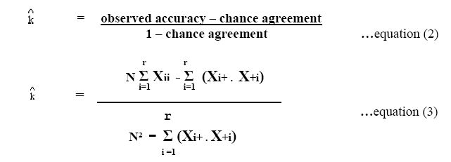
Accuracy estimation in terms of producer's accuracy, user's accuracy, overall accuracy and Kappa coefficient were subsequently made after generating confusion matrix. The Kappa coefficient is a measure of the difference between the actual agreement between reference data and an automated classifier and the chance agreement between the reference data and the random classifier as shown in equation (1) and equation (2). This statistics serves as an indicator of the extent to which the percentage correct values of an error matrix are due to “true” agreement versus “chance” agreement. It incorporates the non-diagonal elements of the error matrix as a product of the row and column diagonal.

Where     r      =    number of rows in the error matrix

             Xii    =    the number of observations in row i and column i (on the major diagonal)

            Xi+   =   total of observations in row i

            X+i  =   total of observations in column i

            N      =   total number of observations included in matrix

Of the three hard supervised classifiers, Maximum likelihood is the best and  computationally difficult.  The forest classes obtained were then identified as evergreen, semi-evergreen, moist deciduous, and dry deciduous.  Temporal change analysis was done  considering the forest cover of Uttara Kannada in 1984. Digitised Forest Map of South India generated by J.P. Pascal of the French Institute, Pondicherry (1984), was compared with the classified image obtained, by overlaying the image on the digitized map. This gave the change in the forest cover and also the forest types over a period of about fifteen years.

Figure 7: NDVI of Uttara Kannada