MODIS NDVI and LST data were used to generate monthly NDVI and monthly temperature maps. Detail documentation of MODIS NDVI compositing process and Quality Assessment Science Data Sets (QASDS) is available at NASA's MODIS web site (MODIS, 1999). MODIS LST products user’s guide documents data generation, data attributes and quality assurance details. LST maps were calibrated and validated from past data records collected by NOAA (http://gis.ncdc.noaa.gov/map/viewer). Monthly rainfall raster maps were obtained by interpolation of point data and the values were validated using rain gauge stations located at several sites in the study area. A small part of the study area as seen in Google Earth (http://earth.google.com) in 2003 is given in figure 3 (a) and in 2012 is given in figure 3 (b) respectively, and figure 3 (c) shows NDVI of January, 2003 and December, 2012 corresponding to the region shown in figure 3 (a) and (b).
(a) January, 2003
(b) December, 2012
Part of Western Ghats (a) and (b) as seen in Google Earth for two different dates.
NDVI (Jan, 2003)
NDVI (Dec, 2012)
(c) NDVI maps of January, 2003 and December 2012 for the corresponding region in (a) and (b).
Figure 3: A small part of the study area (a) and (b) as seen in Google Earth in 2003 and 2012; (c) NDVI of the same region in January, 2003 and December, 2012.
5.1 Time-series MODIS NDVI based LC change analysis from 2003 to 2012
MODIS NDVI time-series and reference data were used for multi-temporal LC analysis and validation. Monthly NDVI values for each 250 m grid cell within the study area (during 2003–2012) were identified that exhibited greater than specified threshold values known as “NDVI class separation threshold” and were labeled as separate LC classes. Boxplots were generated to understand the variability and to visualize the separation of classes through their statistical properties such as median and inter-quartile range for each class. The ambiguities in separation between two different LC classes due to seasonal differences were resolved by adjusting the NDVI class separation threshold and expert knowledge. Figure 4 shows variations (boxplots) for the four LC classes – dense vegetation, agriculture/grassland, soil/settlement and water for January, 2003 and December, 2012 respectively for northern Western Ghats.
January, 2003
December, 2012
Figure 4: Boxplots for dense vegetation, agriculture/grassland, soil/settlement and water for the year January, 2003 and December, 2012 for northern Western Ghats (X-axis: Month, Y-axis: NDVI values).
Boxplots helped in visualizing the separability of LC classes through NDVI. Their inter-quartile range and whiskers aided in assessing the overlapping regions between classes which further helped in adjusting the NDVI thresholds for different LC classes, for each month and different years. The boxplots show that LC classes were separable and NDVI thresholding was successful in delineating the LC classes from multi-temporal NDVI images. Similarly, the four LC classes were also separated for central and southern Western Ghats based on monthly NDVI thresholding from 2003 to 2012 that have not been shown here. The LC maps were validated in various ways –
By overlaying test data obtained using GPS and field survey.
By comparison with limited number of temporal high resolution classified images (Landsat ETM+ available in public domain and IRS LISS III/IV images procured from NRSC – National Remote Sensing Centre, Hyderabad, India).
By visual inspection/expert knowledge, and
By comparing each of the LC classes with Google Earth historical images (http://earth.google.com) through visual checks.
However, the error matrices have not been shown here because of the large spatial and temporal nature of the data. The producer's accuracies ranged from 67 to 81%, user's accuracies ranged from 69 to 84% and overall accuracies ranged between 65 to 80.5%. Figure 5 shows sample LC maps of January 2003 and December 2012 for northern, central and southern Western Ghats and table 1–3 depicts the LC class statistics. Figure 6–8 shows time-series graph for the LC change (dense vegetation and agriculture) for northern, central and southern Western Ghats.
Northern Western Ghats (January, 2003)
Northern Western Ghats (December, 2012)
Central Western Ghats (January, 2003)
Central Western Ghats (December, 2012)
Southern Western Ghats (January, 2003)
Southern Western Ghats (December, 2012)
Figure 5: LC maps of northern, central and southern Western Ghats of January, 2003 and December, 2012. Table 1: LC change statistics of northern Western Ghats from 2003 to 2012 based on NDVI classification
Month-Year
Dense Vegetation
Agriculture/ grassland
Soil/settlement
Water
ha
%
ha
%
ha
%
ha
%
Jan-03
2340719
23.64
7315449
73.88
108282.6
1.09
138085.2
1.39
Jan-04
2276359
22.99
7356046
74.29
128151
1.29
142058.9
1.43
Jan-05
2233782
22.56
7404565
74.78
131131.2
1.32
133118.1
1.34
Jan-06
2196157
22.18
7434270
75.08
126164.1
1.27
146032.5
1.47
Jan-07
2177344
21.99
7421201
74.95
166894.3
1.68
137091.8
1.38
Jan-08
2164373
21.86
7448133
75.22
177821.9
1.79
116230
1.17
Jan-09
2146649
21.68
7420408
74.94
168881.1
1.7
166894.3
1.68
Jan-10
2133974
21.55
7505563
75.80
147025.9
1.48
115236.6
1.16
Jan-11
2119023
21.40
7478828
75.53
177821.9
1.79
137091.8
1.38
Jan-12
2106053
21.27
7509524
75.84
169874.5
1.71
117223.4
1.18
Dec-12
2059516
20.80
7536259
76.11
182789
1.84
123183.9
1.24
Table 2: LC change statistics of central Western Ghats from 2003 to 2012 based on NDVI classification
Month-Year
Dense Vegetation
Agriculture/ grassland
Soil/settlement
Water
ha
%
ha
%
ha
%
ha
%
Jan-03
5073131
53.39
4331023
45.58
4751
0.05
93119.6
0.98
Jan-04
5031322
52.95
4368081
45.97
6651.4
0.07
95970.2
1.01
Jan-05
4981957
52.43
4402288
46.33
17103.6
0.18
95970.2
1.01
Jan-06
4956754
52.17
4435545
46.68
17103.6
0.18
95020
1
Jan-07
4940102
51.99
4471653
47.06
9502
0.1
76966.2
0.81
Jan-08
4876439
51.32
4502059
47.38
27555.8
0.29
86468.2
0.91
Jan-09
4851733
51.06
4550520
47.89
20904.4
0.22
78866.6
0.83
Jan-10
4834630
50.88
4564773
48.04
19004
0.2
85518
0.9
Jan-11
4806175
50.58
4598980
48.4
19954.2
0.21
76966.2
0.81
Jan-12
4709168
49.56
4684498
49.3
33257
0.35
73165.4
0.77
Dec-12
4656546
49.01
4741510
49.9
49410.4
0.52
56061.8
0.59
Table 3: LC change statistics of southern Western Ghats from 2003 to 2012 based on NDVI classification
Month-Year
Dense Vegetation
Agriculture/ grassland
Soil/settlement
Water
ha
%
ha
%
ha
%
ha
%
Jan-03
5897318
78.78
1538333
20.55
7485.81
0.1
42669.09
0.57
Jan-04
5839677
78.01
1593728
21.29
7485.81
0.1
44914.84
0.6
Jan-05
5755243
76.88
1636397
21.86
6737.23
0.09
44914.84
0.6
Jan-06
5664509
75.67
1721735
23
6737.23
0.09
44914.84
0.6
Jan-07
5621840
75.1
1811565
24.2
6737.23
0.09
45663.42
0.61
Jan-08
5564948
74.34
1867709
24.95
6737.23
0.09
45663.42
0.61
Jan-09
5541742
74.03
1893909
25.3
4491.48
0.06
45663.42
0.61
Jan-10
5531262
73.89
1908881
25.5
8982.97
0.12
36680.45
0.49
Jan-11
5508056
73.58
1923104
25.69
5988.64
0.08
48657.74
0.65
Jan-12
5483353
73.25
1951550
26.07
5240.06
0.07
45663.42
0.61
Dec-12
5465387
73.01
1976253
26.4
8982.97
0.12
35183.29
0.47
Sometimes, it was difficult to segregate dense vegetation from agriculture/grassland by identifying an exact NDVI threshold, and exposed soil covered with grass created confusion between soil and grassland. Table 1–3 shows that forest area have decreased by ~3% in northern, by ~4.4% in central and by 5.7% in southern Western Ghats. Agriculture/grasslands have increased by 2.23% in northern, by 4.3% in central and 5.8% in southern region respectively. Soil/settlement have increased marginally and the spatial extent of water bodies have decreased in all the three regions of Western Ghats. Figure 6–8 show percentage change in the estimate of dense vegetation and agriculture/grassland in northern, central and southern Western Ghats from 2003 to 2012. Northern and central Western Ghats shows very similar trends. Dense vegetation/forest area increases in September–October–November and decreases in January–February. This season (August–September–October) corresponds from mid to end of the monsoon that brings heavy showers from Arabian Sea. Due to this rain, entire Ghats region is full of thick vegetation. Agriculture/grassland area is maximum in August–September and December–January and minimum in April–May in both northern and central Western Ghats. However, southern Western Ghats shows a slightly different pattern with peak dense vegetation between October through June and lowest in August and September. Agriculture crops occupy maximum spatial extent between August to December and show valleys in the time-series graph between April to June.
The valleys in the three graphs (figure 6 to 8) for all the three climatic/ecological regions for agriculture correspond to April to June when there is no water and the farmlands are generally fallow. The farmers wait for the monsoon in July/August to sow the crops. Crops mature and are ready for harvesting in December/January indicating peak in the graphs with maximum area under this class (agriculture). These crops are popularly known as kharif crops or monsoon crops (July to October) and rabbi crops (October to March). Southern Western Ghats receives the first rainfall of monsoon season in the country every year and therefore agriculture/grassland areas show an early increasing trend in this region. It is to be noted that the data for July month was not available (due to the presence of clouds), therefore the graph suddenly dips down in this month for all the years. Figure 6–8 brings a very important conclusion, i.e. the total dense green area in northern and central Western Ghats are between 20–80% of all the LC classes while dense vegetation constitute around 60–95% of the southern Western Ghats throughout the years of study (2003–2012).
Figure 6: Percentage change (monthly) in dense vegetation and agriculture/grassland in northern Western Ghats from 2003 to 2012. Figure 7: Percentage change (monthly) in dense vegetation and agriculture/grassland in central Western Ghats from 2003 to 2012. Figure 8: Percentage change (monthly) in dense vegetation and agriculture/grassland in southern Western Ghats from 2003 to 2012.
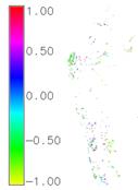
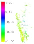
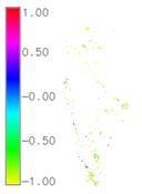
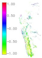
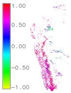
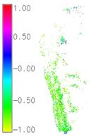
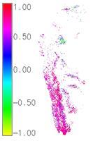
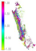
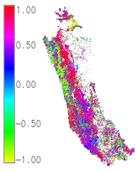
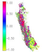
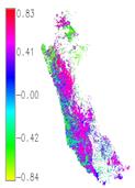
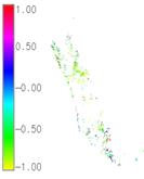
Figure 9–11 show changes in dense vegetation/forest (left figure) and agriculture/grassland (right figure) to other LC classes. The changes are represented by different colours for a year. For example, in figure 9, yellow in the legend shows areas that have been converted from dense vegetation to either agriculture or grassland or soil/settlement or water in 2003 (in the left figure). Whereas red pixels in the right figure shows areas that have been converted from either dense vegetation, or soil/settlement or other classes to agriculture/grassland in 2004. Similarly, figures 10 and 11 reflect the changes in central and southern Western Ghats. Table 4 shows area converted from dense vegetation to other three classes, and from other three classes to agriculture/grassland in the three regions of Western Ghats. It indicates the area (in ha) that have changed from dense vegetation class to other LC classes (agriculture, soil or water) from January, 2003 to December, 2003 and then for each subsequent year (2004 to 2012). It may be noted that the total area belonging to dense vegetation class is decreasing every year indicating "forest loss" although there might be pixels belonging to other three classes that would also have changed to dense vegetation class at other pixel locations but may be present in low numbers (counts) in the entire image. Minus sign indicates loss in overall forest area every year. The remaining part of the table shows annual conversion from other classes (dense vegetation, soil/settlement and water) to agriculture/grassland indicated by positive sign. It signifies that overall, agricultural area is increasing at the cost of other three LC classes.
Figure 9: Annual change from one LC class to other LC classes in northern Western Ghats between 2003 to 2012 obtained from MODIS NDVI. The base image (background) is 250 m black and white version of MODIS NDVI of January, 2003. Colour palate in the middle represents changes in that year. Figure 10: Annual change from one LC class to other LC classes in central Western Ghats between 2003 to 2012 obtained from MODIS NDVI. The base image (background) is 250 m black and white version of MODIS NDVI of January, 2003. Colour palate in the middle represents changes in that year. Figure 11: Annual change from one LC class to other LC classes in southern Western Ghats between 2003 to 2012 obtained from MODIS NDVI. The base image (background) is 250 m black and white version of MODIS NDVI of January, 2003. Colour palate in the middle represents changes in that year.
Table 4: Annual conversion from dense vegetation to other LC classes, and from other LC classes to agricultural/grassland in the three regions of Western Ghats.
Annual conversion from dense vegetation to other classes (agriculture/grassland, soil/settlement and water)
From year – To year
Northern Western Ghats (area in ha)
Central Western Ghats (area in ha)
Southern Western Ghats (area in ha)
January, 2003 – January, 2004
-64360
-41809
-57641
January, 2004 – January, 2005
-42577
-49365
-84435
January, 2005 – January, 2006
-37625
-25203
-90733
January, 2006 – January, 2007
-18813
-16652
-42669
January, 2007 – January, 2008
-12971
-63663
-56892
January, 2008 – January, 2009
-17724
-24706
-23206
January, 2009 – January, 2010
-12675
-17103
-10480
January, 2010 – January, 2011
-14951
-28455
-23206
January, 2011 – January, 2012
-12970
-97007
-24703
January, 2012 – December, 2012
-46537
-52622
-17966
Annual conversion from other classes (dense vegetation, soil/settlement and water) to agriculture/grassland
Figure 12–14 shows monthly boxplots for dense vegetation, agriculture/grassland, soil/settlement and water for the year 2003 and 2012 for northern, central and southern Western Ghats (X-axis: Month, Y-axis: NDVI values). In general, median of all the boxplots of dense vegetation class (figure 12 and 13 for 2003 and 2012) is different for northern and central Western Ghats. However, the locations of median are closer for a few consecutive months (for example, February–March, September–October) in southern Western Ghats and their trends (figure 14) for 2003 and 2012 are alike with overlapping inter-quartile range. For all the three regions of Western Ghats, median NDVI is low during March to June, which corresponds to the summer season and the leaves have either dried or fallen. In September– November, median NDVI is higher compared to other months; this is also evident from the graphs in figure 6, 7 and 8 showing percentage change in dense vegetation from 2003 to 2012 and from monthly minimum, maximum and mean NDVI values for dense vegetation for northern, central and southern Western Ghats in figure 15.
Agriculture shows a similar trend like dense vegetation; they have different medians for all the months, yet the median follows similar trend across the months in a year in northern and central Western Ghats (see figure 12 and 13). April–May–June have lowest median when the crops are being sown at the beginning of monsoon with smallest box and inter-quartile range and highest median in September to November which is the time before harvesting of crops (matured/grownup state). This observation is also supported by the change in LC statistics in figure 6 and 7.
Southern Western Ghats presents a slightly different picture with a dissimilar trend as that of other two regions, although they follow a similar yearly trend across months in 2003 and 2012 which are multimodal and non-sinusoidal (figure 15) with overlapping inter-quartile ranges (see figure 14). The peak season for agricultural crops is August to December and have lowest median in March–April–May. This may indicate early summer and early onset of monsoon in this region. LC change statistics in figure 8 further corroborates this trend.
Soil/settlements have minimum NDVI in May/June (summer) and have maximum NDVI (towards positive) in November–January. For southern Western Ghats, minimum NDVI for soil occurs in May and maximum occurs during August to December, earlier than northern and central regions. Water bodies exhibit least NDVI from April to June as they are either dry or have less water and have maximum NDVI in August (monsoon) with plenty of rain water in rivers/streams, water accumulated in lakes and sometimes covered with macrophytes.
Dense vegetation (2003)
Dense vegetation (2012)
Agriculture/grassland (2003)
Agriculture/grassland (2012)
Soil/settlement (2003)
Soil/settlement (2012)
Water (2003)
Water (2012)
Figure 12: Boxplots for dense vegetation, agriculture/grassland, soil/settlement and water for the year 2003 and 2012 for northern Western Ghats (X-axis: Month, Y-axis: NDVI values).
Dense vegetation (2003)
Dense vegetation (2012)
Agriculture/grassland (2003)
Agriculture/grassland (2012)
Soil/settlement (2003)
Soil/settlement (2012)
Water (2003)
Water (2012)
Figure 13: Boxplots for dense vegetation, agriculture/grassland, soil/settlement and water for the year 2003 and 2012 for central Western Ghats (X-axis: Month, Y-axis: NDVI values).
Dense vegetation (2003)
Dense vegetation (2012)
Agriculture/grassland (2003)
Agriculture/grassland (2012)
Soil/settlement(2003)
Soil/settlement (2012)
Water (2003)
Water (2012)
Figure 14: Boxplots for dense vegetation, agriculture/grassland, soil/settlement and water for the year 2003 and 2012 for southern Western Ghats (X-axis: Month, Y-axis: NDVI values).
Statistical analysis showed that the above boxplots are not exactly symmetrical about median, hence sample mean does not coincide with sample median. Therefore median does not necessarily represent the trend of LC classes for further analysis, so we explore the utility of minimum-mean-maximum time-series NDVI values of dense vegetation and subsequently study the different LC classes using mean NDVI.
Figure 15 depicts monthly minimum, mean and maximum NDVI time-series values for dense vegetation for the northern, central and southern Western Ghats (top, middle and bottom graphs) from 2003 to 2012. The trend line almost shows a sinusoidal wave pattern with peak NDVI values in August–February and valley in April–June in northern and central Western Ghats. Southern Western Ghats shows a slightly different pattern with maximum NDVI depicted by high peak (close to +1 NDVI values) most of the months in a year. It shows high mean NDVI between September–January and low NDVI values between March to June (in summer months) every year.
A comparison of NDVI values with the spatial extent graphs in figure 6–8 reveal that northern and central Western Ghats show maximum spatial extent under dense vegetation in September–November whereas peak NDVI is present from August to January. The peak NDVI may also be contributed from the agricultural crops which are in their growing stage in September and in matured stage in December. They are harvested in December/January, bringing down the spatial extent in January–February while the reflectance from dense green forest may still exhibit high NDVI values till February.
In southern Western Ghats, spatial extent of dense vegetation is maximum during October to June while the peak NDVI reflectance is from September to January. This indicates that forest and agricultural crops (that also include coconut, rubber, coffee plantation, etc.) mature during September to January exhibiting high mean NDVI, while the geographical extent of combined forest and agricultural crops remain high through October to June. One reason for this could be that, the contribution from vegetation and agricultural crops to high reflectance in NIR band could be least after harvesting (in February), thereby decreasing the overall mean NDVI. On the other hand, agriculture crops have a low geographical extent among green vegetation and the southern Western Ghats is mostly dominated by dense mixed vegetation. So, even though the mean NDVI forms a valley after harvesting (in February), the overall dense vegetation continue to show higher spatial extent till June across years. This phenomenon is observed as a repeated cycle every year during the course of this study. It also indicates that during the growth stage of the plants in September to January, it is difficult to separate the dense agricultural crops from dense vegetation by means of NDVI and high spectral resolution sensors with higher number of spectral bands such as Hyper-spectral data may be required for further classification of different vegetation types. From the above discussion and also reported by Lunetta et al., (2006), we see that minimum and maximum NDVI values mainly aid in separation of LC classes. Therefore mean NDVI values of different LC classes (Aguilar et al., 2012; Mao et al., 2012; Raynolds et al., 2008) are explored further in analyzing the behaviour of different LC classes.
Figure 15: Monthly minimum, mean and maximum NDVI values for dense vegetation for the northern, central and southern Western Ghats (top, middle and bottom graphs in the figure).
Figure 16 shows temporal mean NDVI profiles for the major end members (dense vegetation, agriculture/grassland, soil/settlement and water bodies) corresponding to the 3 (northern, central and southern) climatic regions of Western Ghats.
Figure 16: Temporal mean NDVI profiles for the major end members corresponding to the 3 (northern, central and southern) climatic regions of Western Ghats (Note: X-axis: Mean NDVI values, Y-axis: Month-Year).
Figure 16 indicates that mean NDVI of dense vegetation and agriculture follow similar patterns in northern and central Western Ghats with peak in monsoon (September–October–November) and valleys in summer (April–May) respectively. Bare soil/settlement have almost constant mean NDVI and have low NDVI values close to 0. Southern Western Ghats shows similar trend like northern and central Western Ghats, however the peaks and valleys are not uniform for dense forest/vegetation and tend to rise during October each year (see figure 16). NDVI values for water tend to increase whenever there is a peak in vegetation across the months and year (in monsoon season) in all the three regions of Western Ghats.
Figure 17: Boxplot of monthly NDVI changes of dense forest for monsoon season (June, August and September) in Western Ghats from 2003 to 2012.
Figure 17 is the boxplot of NDVI changes for forest class in June, August and September (monsoon season) for northern, central and southern Western Ghats from 2003 to 2012. It is shown that the median of the boxplot follow a somewhat sinusoidal pattern in each month in northern and central Western Ghats from 2003 to 2012. For southern Western Ghats, the pattern in the median has less deviation across the years. The noticeable points here are:
In northern Western Ghats, 2005, 2006, and 2010 shows higher median values (ranging approximately from 0.5 to 0.7) compared to 2003 and 2011 that have the lesser NDVI inter-quartile range for June (median is ~0.5).
For central Western Ghats, 2003–4 and 2011–12 show lesser median in the month of June than in the middle years.
In central Western Ghats, 2008 has least median (~0.5–0.55) for August for both northern and central Western Ghats indicating lesser vegetation; the reason for this may be attributed to the climatic and physical factors. The median in September is generally higher in the year 2006, 2009 and 2012 than other two months (June and August) in both the regions showing more greenery than other years.
Particularly, southern Western Ghats shows higher NDVI values for all three months for all the years (2003 to 2012) compared to northern and central Western Ghats indicating more greenery and this trend is static. For all the other months (except monsoon season), the records show static patterns.
Figure 18 shows summary trend maps of NDVI changes in northern, central and southern Western Ghats from 2003 to 2012 calculated from monthly NDVI time-series. It is to be noted that the NDVI differencing values can range from +2 to -2 for the difference image. For example, Map1 and Map 2 can have NDVI value range from +1 to -1. Extreme changes in NDVI can result from pixels subtracting -1 from +1 (i.e. +1 - (-1)) which is +2 where the actual change is negative and decreasing value from +1 to -1, so should be shown as -2. The difference pixel can also result from subtracting +1 from -1 (i.e. -1 - (1)) which is -2 where the actual change is positive and increasing from -1 to +1, so should be shown as +2. Therefore, the difference values are multiplied by -1 to show the actual magnitude and direction of the change in differences.
Figure 18 indicates different pattern for northern, central and southern regions. Major changes from 2003 to 2012 have taken place in the 0.0 to 0.1 (grey) and 0 to -0.3 (pink) followed by 0.1 to 0.2 (green) in northern Western Ghats. In central and southern regions, major changes have taken between 0 to -0.3 (pink) followed by 0 to 0.1 (grey) with a marginal change between 0.1 to 0.2 (green). Table 5 shows the LC change statistics in Western Ghats based on NDVI differencing. NDVI difference ranges with large change are highlighted in shaded rows corresponding to graphs in figure 18.
Table 5: LC change statistics of Western Ghats from 2003 to 2012 based on NDVI differencing
Northern Western Ghats
Central Western Ghats
Southern Western Ghats
NDVI differencing range
Area
NDVI differencing range
Area
NDVI differencing range
Area
ha
%
ha
%
ha
%
-0.76 - -0.3
14740
0.16
-0.80 - -0.3
15249
0.17
-1.8 - -0.3
16545
0.24
-0.3-0.0
2272093
25.1
-0.3-0.0
6804193
77.1
-0.3-0.0
4426429
64.31
0.0-0.10
5671090
62.64
0.0-0.10
1864756
21.13
0.0-0.10
2206011
32.05
0.10-0.20
1038850
11.47
0.10-0.20
119077
1.35
0.10-0.20
188560
2.74
0.20-0.40
55858
0.62
0.20-0.40
19707
0.22
0.20-0.40
37274
0.54
0.40-0.84
1180
0.01
0.40-0.80
1994
0.02
0.40-1
8273
0.12
Total
9053811
100
8824976
100
6883092
100
Figure 18: Summary trend maps of NDVI changes in Western Ghats from 2003 to 2012 calculated from monthly (January and December) NDVI time-series.
Many research results show that changes in vegetation are seriously influenced by temperature and precipitation. For example, Li et al. (2002) observed that a significant correlation exist between NDVI and eco-climatic parameters, and that NDVI growing degree days correlation was stronger than NDVI–rainfall correlation. These studies presented reasonable and reliable conclusions regarding NDVI changes and the relationship between vegetation NDVI and climatic parameters.
Figure 19–21 shows sample temperature maps (in °C) computed for northern, central and southern Western Ghats from January to December 2003 and 2012. Figure 22 shows minimum, mean and maximum temperature of the three regions.
January, 2003
February, 2003
March, 2003
April, 2003
May, 2003
June, 2003
August, 2003
September, 2003
October, 2003
November, 2003
December, 2003
January, 2012
February, 2012
March, 2012
April, 2012
May, 2012
June, 2012
August, 2012
September, 2012
October, 2012
November, 2012
December, 2012
Figure 19: Sample monthly temperature maps (in °C) for 2003 and 2012 for northern Western Ghats. Images of June and August had lot of pixels with cloud cover, so these images have many no data values (white in colour). (Note: July temperature map was not computed due to presence of cloud in the data.)
January, 2003
February, 2003
March, 2003
April, 2003
May, 2003
June, 2003
August, 2003
September, 2003
October, 2003
November, 2003
December, 2003
January, 2012
February, 2012
March, 2012
April, 2012
May, 2012
June, 2012
August, 2012
September, 2012
October, 2012
November, 2012
December, 2012
Figure 20: Monthly temperature maps (in °C) for 2003 and 2012 for central Western Ghats. Images of June and August had lot of pixels with cloud cover, so these images have many no data values (white in colour). (Note: July temperature map was not computed due to presence of cloud in the data.)
January, 2003
February, 2003
March, 2003
April, 2003
May, 2003
June, 2003
August, 2003
September, 2003
October, 2003
November, 2003
December, 2003
January, 2012
February, 2012
March, 2012
April, 2012
May, 2012
June, 2012
August, 2012
September, 2012
October, 2012
November, 2012
December, 2012
Figure 21: Monthly temperature maps (in °C) for 2003 and 2012 for southern Western Ghats. Images of June and August had lot of pixels with cloud cover, so these images have many no data values (white in colour). (Note: July temperature map was not computed due to presence of cloud in the data.)
Figure 22: Monthly minimum, mean and maximum temperature (in °C) of the three regions (top - northern, middle - central and bottom - southern Western Ghats). [X-axis: Month-Year, Y-axis: temperature (in °C)].
Figure 22 shows that minimum, mean and maximum temperature, which almost follow a wave like pattern with peak summer temperature (14–42 °C) in April–May–June every year and lowest winter temperature (7–38 °C) in December–January (shown in blue dotted line) in northern and central Western Ghats. Southern Western Ghats shows a slightly different pattern with maximum variance in temperature in December–January months and highest temperature in summer (March–April–May) each year. There is not much variability between summer (11–39 °C) and winter temperatures ranges (8–35 °C). Figure 23 shows mean monthly temperature ± standard deviation graph further highlighting the temperature variation trend.
Figure 23: Mean monthly temperature ± standard deviation (in °C) for northern, central and southern Western Ghats (top - northern, middle - central and bottom - southern Western Ghats) X-axis: Month-Year, Y-axis: temperature (in °C)
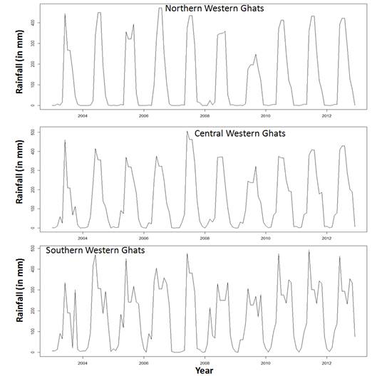
Figure 24–26 shows sample rainfall maps (in mm) for northern, central and southern Western Ghats from January to December 2003 and 2012.
January, 2003
February, 2003
March, 2003
April, 2003
May, 2003
June, 2003
July, 2003
August, 2003
September, 2003
October, 2003
November, 2003
December, 2003
January, 2012
February, 2012
March, 2012
April, 2012
May, 2012
June, 2012
July, 2012
August, 2012
September, 2012
October, 2012
November, 2012
December, 2012
Figure 24: Monthly rainfall maps (in mm) for 2003 and 2012 for northern Western Ghats.
January, 2003
February, 2003
March, 2003
April, 2003
May, 2003
June, 2003
July, 2003
August, 2003
September, 2003
October, 2003
November, 2003
December, 2003
January, 2012
February, 2012
March, 2012
April, 2012
May, 2012
June, 2012
July, 2012
August, 2012
September, 2012
October, 2012
November, 2012
December, 2012
Figure 25: Monthly rainfall maps (in mm) for 2003 and 2012 for central Western Ghats.
January, 2003
February, 2003
March, 2003
April, 2003
May, 2003
June, 2003
July, 2003
August, 2003
September, 2003
October, 2003
November, 2003
December, 2003
January, 2012
February, 2012
March, 2012
April, 2012
May, 2012
June, 2012
July, 2012
August, 2012
September, 2012
October, 2012
November, 2012
December, 2012
Figure26: Monthly rainfall maps (in mm) for 2003 and 2012 for southern Western Ghats.
Figure 27–29 shows total annual rainfall for the three regions. It is evident from the figures that the coastal areas receive highest rainfall and its intensity decreases towards the eastern side in the central and southern Western Ghats. The areas that receive lesser rainfall (called the rain shadow area) are often plains where agriculture is practiced. The rain fed areas have undulating terrain with mix of evergreen to semi-evergreen forest that regulates the regional temperatures between 22 to 32 °C. In southern Western Ghats, plantation is practiced in the hilly areas.
2003
2004
2005
2006
2007
2008
2009
2010
2011
2012
Figure 27: Total annual rainfall (in mm) for northern Western Ghats from 2003 to 2012 with rain gauge stations overlaid.
2003
2004
2005
2006
2007
2008
2009
2010
2011
2012
Figure 28: Total annual rainfall (in mm) for central Western Ghats from 2003 to 2012 with rain gauge stations overlaid.
2003
2004
2005
2006
2007
2008
2009
2010
2011
2012
Figure29: Total annual rainfall (in mm) for southern Western Ghats from 2003 to 2012 with rain gauge stations overlaid.
Figure 30–32 shows mean monthly temperature (Y-axis in °C) and monthly rainfall (secondary Y-axis in mm) for northern, central and southern Western Ghats respectively. Table 6–8 details monthly mean (µ) ± standard deviation (σ) of NDVI, LST and rainfall for forest and agriculture/grassland (2003 and 2012) for northern, central and southern Western Ghats with missing data indicated with "--". Appendix 1 details mean NDVI, LST and rainfall for all the months and year for both the classes. Northern and central Western Ghats typically experience high rainfall (~ 450 to 500 mm) during June to September each year with 2009 receiving lowest rainfall among all the years as seen in figure 30 and 31. The mean temperature almost follows a cyclic pattern (with higher standard deviation), and extreme summer temperatures in April–May with minimum and maximum temperature between 20 to 35 °C in northern Western Ghats and 18 to 30 °C in central Western Ghats. Southern Western Ghats has early onset of the monsoon with highest rainfall in June every year and hottest days during April to May with lower temperature variations across the year (23° to 30° C) as shown in figure 32.
Figure 30: Mean monthly temperature (Y-axis in °C) and monthly rainfall (secondary Y-axis in mm) for northern Western Ghats. Figure 31: Mean monthly temperature (Y-axis in °C) and monthly rainfall (secondary Y-axis in mm) for central Western Ghats. Figure 32: Mean monthly temperature (Y-axis in °C) and monthly rainfall (secondary Y-axis in mm) for southern Western Ghats.
Table 6: Mean (µ) ± standard deviation (σ) of NDVI, LST and rainfall for forest and agriculture/grassland class for northern Western Ghats
Month, Year
NDVI (µ ± σ)
LST (µ ± σ)
rainfall (µ ± σ)
Month, Year
NDVI (µ ± σ)
LST (µ ± σ)
rainfall (µ ± σ)
Forest
Jan, 2003
0.59 ± 0.07
21 ± 4
0.23 ± 0.41
Jan, 2012
0.58±0.06
18.18±2
1.5±2
Feb, 2003
0.52 ± 0.08
22 ± 3
0.03 ± 0.04
Feb, 2012
0.52±0.07
22.07±3
0.3±0
Mar, 2003
0.41 ± 0.09
25.96 ± 3.3
7.02 ± 0.78
Mar, 2012
0.42±0.09
25.93±3
1.6±1
Apr, 2003
0.39 ± 0.10
29.95 ± 4
1.18 ± 2.47
Apr, 2012
0.40±0.1
29.45±3
5.7±6
May, 2003
0.4 ± 0.11
29.02 ± 4
17.74 ± 8
May, 2012
0.41±0.1
30.17±3
5.3±7
Jun, 2003
0.4 ± 0.1
23.31 ± 5
444 ± 145
Jun, 2012
0.41±0.1
28.33±3
391.0±84
Aug, 2003
0.63 ± 0.09
27.50 ± 2
266 ± 72
Aug, 2012
0.60±0.07
25.66±1
421.8±48
Sep, 2003
0.69 ± 0.10
25.27 ± 1
169 ± 35
Sep, 2012
0.67±0.09
24.35±2
284.2±135
Oct, 2003
0.68 ± 0.1
29.43 ± 2
46.42 ± 17
Oct, 2012
0.68±0.09
22.93±3
127.8±60
Nov, 2003
0.62 ± 0.1
23 ± 3
6.09 ± 2.65
Nov, 2012
0.63±0.08
19.37±2
78.0±26
Dec, 2003
0.6 ± 0.1
19.56±2.83
0.00 ± 0.01
Dec, 2012
0.61±0.09
18.14±3
0.9±1
Agriculture/grassland
Jan, 2003
0.34 ± 0.08
22 ± 3
0.51 ± 0.74
Jan, 2012
0.35 ± 0.1
21.43 ± 3
2 ± 2.09
Feb, 2003
0.3 ± 0.07
23 ± 4
0.03 ± 0.06
Feb, 2012
0.31 ± 0.1
26.76 ± 4
0.35 ± 0.3
Mar, 2003
0.24 ± 0.03
30.77 ± 3
7.35 ± 0.94
Mar, 2012
0.24
30.26 ± 3
2.22 ± 1
Apr, 2003
0.22 ± 0.03
34.56 ± 3
0.61 ± 1.79
Apr, 2012
0.22
33.5 ± 3
3.61 ± 5.5
May, 2003
0.22 ± 0.03
33.75 ± 3
24.81 ± 9.9
May, 2012
0.22
33.9 ± 2
4.74 ± 3
Jun, 2003
0.22
30.06 ± 5.5
402 ± 109
Jun, 2012
0.22
31.96 ± 3
295.3 ± 83
Aug, 2003
0.37 ± 0.09
27.95 ± 2.1
260 ± 66.6
Aug, 2012
0.34 ± 0.1
26.67 ± 2
398.7 ± 56
Sep, 2003
0.37 ± 0.09
27.31 ± 2
160 ± 31
Sep, 2012
0.37 ± 0.1
26.14 ± 3
231 ± 114
Oct, 2003
0.37 ± 0.09
32.78 ± 1.5
43.67 ± 21
Oct, 2012
0.41 ± 0.1
29.4 ± 3
87.95 ± 35
Nov, 2003
0.37 ± 0.08
26.5 ± 3.5
7.18 ± 2.20
Nov, 2012
0.39 ± 0.1
23.78 ± 3
76.16 ± 19
Dec, 2003
0.36 ± 0.08
23.54 ± 3.6
0
Dec, 2012
0.37 ± 0.1
23.08 ± 4
0.70 ± 1
Table 7: Mean (µ) ± standard deviation (σ) of NDVI, LST and rainfall for forest and agriculture/grassland class for central Western Ghats
Month, Year
NDVI (µ ± σ)
LST (µ ± σ)
rainfall (µ ± σ)
Month, Year
NDVI (µ ± σ)
LST (µ ± σ)
rainfall (µ ± σ)
Forest
Jan, 2003
0.65 ± 0.11
17 ± 4
0.81 ± 1.26
Jan, 2012
0.65 ± 0.1
15.9 ± 4
9.21 ± 2.7
Feb, 2003
0.53 ± 0.15
22 ± 5
0.66 ± 1.04
Feb, 2012
0.53 ± 0.2
22.8 ± 5
0.66 ± 0.6
Mar, 2003
0.50 ± 0.16
25.81 ± 3.4
10.74 ± 1
Mar, 2012
0.51 ± 0.2
24.98 ± 3
4.83 ± 4
Apr, 2003
0.51 ± 0.17
26.78 ± 3.4
58.4 ± 37
Apr, 2012
0.52 ± 0.2
26.15 ± 3
66 ± 34
May, 2003
0.50 ± 0.16
29.92 ± 4
25.67 ± 7
May, 2012
0.55 ± 0.2
26.86 ± 4
78 ± 31
Jun, 2003
0.52 ± 0.12
25.76 ± 2.9
459 ± 308
Jun, 2012
0.52 ± 0.1
28 ± 2.4
407 ± 107
Aug, 2003
0.62 ± 0.1
24.48 ± 1.1
209 ± 115
Aug, 2012
0.62 ± 0.1
26 ± 1.9
429 ± 87
Sep, 2003
0.72 ± 0.11
23.9 ± 1.98
67.87 ± 20
Sep, 2012
0.69 ± 0.1
19.9 ± 2
286 ± 110
Oct, 2003
0.72 ± 0.11
21.5 ± 1.85
112 ± 46.7
Oct, 2012
0.71 ± 0.1
22 ± 2.88
201 ± 52
Nov, 2003
0.69 ± 0.11
20 ± 5
16.7 ± 10.3
Nov, 2012
0.69 ± 0.1
17.99 ± 5
189 ± 48
Dec, 2003
0.67 ± 0.1
18.23 ± 3.6
0.43 ±0.49
Dec, 2012
0.67 ± 0.1
19.8 ± 4
6.86 ± 7
Agriculture/grassland
Jan, 2003
0.34 ± 0.07
24 ± 4
1.67 ± 1.76
Jan, 2012
0.36
23 ± 3.9
8.27 ± 2.4
Feb, 2003
0.27 ± 0.03
29 ± 4
0.84 ± 1.22
Feb, 2012
0.27
31 ± 3.4
0.67 ± 0.5
Mar, 2003
0.25 ± 0.03
31.5 ± 3.78
11.13 ± 1.1
Mar, 2012
0.25
28 ± 2.7
3.2 ± 3.92
Apr, 2003
0.23 ± 0.02
31.86 ± 3
51.83 ± 27
Apr, 2012
0.24
29.5 ± 37
51.5 ± 33
May, 2003
0.23 ± 0.03
36 ± 2
22.7 ± 6.18
May, 2012
0.23
35.47 ± 3
59.1 ± 26
Jun, 2003
0.26 ± 0.04
30 ± 4.9
243 ± 167
Jun, 2012
0.26
31 ± 3.1
343 ± 97
Aug, 2003
0.34 ± 0.09
24.51 ± 1.2
179 ± 100
Aug, 2012
0.35 ± 0.1
25.9 ± 2
376 ± 108
Sep, 2003
0.35 ± 0.09
27.29 ± 2.6
51 ± 20
Sep, 2012
0.37 ± 0.1
23 ± 3.9
195 ± 115
Oct, 2003
0.36 ± 0.08
26.88 ± 3.5
85.26 ± 49
Oct, 2012
0.4 ± 0.07
28 ± 4.7
135 ± 35
Nov, 2003
0.4 ± 0.07
26 ± 3.29
7.08 ± 7.08
Nov, 2012
0.42 ± 0.1
24.6 ± 4
138.9 ± 51
Dec, 2003
0.38 ± 0.07
24 ± 3.57
0.39 ± 0.5
Dec, 2012
0.4 ± 0.06
25.5 ± 3
4.1 ± 6.85
Table 8: Mean (µ) ± standard deviation (σ) of NDVI, LST and rainfall for forest and agriculture/grassland class for southern Western Ghats
Month, Year
NDVI (µ ± σ)
LST (µ ± σ)
rainfall (µ ± σ)
Month, Year
NDVI (µ ± σ)
LST (µ ± σ)
rainfall (µ ± σ)
Forest
Jan, 2003
0.69 ± 0.1
27 ± 2
6.6 ± 2.53
Jan, 2012
0.69 ± 0.1
28.2 ± 2.7
16.6 ± 11
Feb, 2003
0.62 ± 0.16
28 ± 3
6.66 ± 5.35
Feb, 2012
0.61 ± 0.2
27.16 ± 3
2.88 ± 1
Mar, 2003
0.61 ± 0.17
29 ± 1.37
14.9 ± 1.56
Mar, 2012
0.6 ± 0.15
28.8 ± 2
22 ± 16.7
Apr, 2003
0.6 ± 0.18
24.7 ± 1.8
91.3 ± 35
Apr, 2012
0.56 ± 0.2
28.9 ± 1.6
101 ± 63
May, 2003
0.55 ± 0.15
30.38 ± 1.4
64.69 ± 38
May, 2012
0.59 ± 0.2
27 ± 3
140 ± 68
Jun, 2003
0.62 ± 0.16
29.3 ± 1.6
336 ± 159
Jun, 2012
0.56 ± 0.1
28.3 ± 1.9
463.1 ± 7
Aug, 2003
0.69 ± 0.1
25.73 ± 1
189.7 ± 73
Aug, 2012
0.68 ± 0.1
26.6 ± 1.2
293 ± 55
Sep, 2003
0.75 ± 0.1
25.96 ± 0.8
21.64 ± 22
Sep, 2012
0.72 ± 0.1
26.1 ± 1.1
232 ± 67
Oct, 2003
0.73 ± 0.1
26 ± 1
300 ± 82
Oct, 2012
0.73 ± 0.1
30.6 ± 1.5
354 ± 94
Nov, 2003
0.74 ± 0.1
26 ± 0.7
13.05 ± 5.7
Nov, 2012
0.74 ± 0.1
27.3 ± 2.3
333 ± 61
Dec, 2003
0.7 ± 0.1
23.6 ± 1.3
4.07 ± 5.27
Dec, 2012
0.72 ± 0.1
27.1 ± 2.6
75 ± 58.6
Agriculture/grassland
Jan, 2003
0.37 ± 0.06
30 ± 2
8.67 ± 1.64
Jan, 2012
0.41 ± 0.1
32.1 ± 1.8
13.6 ± 11
Feb, 2003
0.27 ± 0.03
32 ± 1
5.04 ± 3.54
Feb, 2012
0.29
31.43 ± 2
2.5 ± 1.1
Mar, 2003
0.25 ± 0.03
30.34 ± 1.2
15.31 ± 0.6
Mar, 2012
0.26
27.15 ± 2
22.4 ± 16
Apr, 2003
0.24 ± 0.02
27.42 ± 2.9
55.36 ± 23
Apr, 2012
0.24
29.74 ± 3
57.7 ± 46
May, 2003
0.23 ± 0.03
29.45 ± 1.9
44.93 ± 24
May, 2012
0.23
35 ± 2
6 ± 3
Jun, 2003
0.28 ± 0.04
29.74 ± 2.7
333.9 ± 80
Jun, 2012
0.28
28.67 ± 2
431 ± 64
Aug, 2003
0.33 ± 0.09
26.06 ± 1.7
191.6 ± 47
Aug, 2012
0.33 ± 0.1
28.8 ± 2.6
273 ± 48
Sep, 2003
0.32 ± 0.09
28.25 ± 1.7
12.23 ± 8.5
Sep, 2012
0.33 ± 0.1
27.5 ± 2.4
157 ± 56
Oct, 2003
0.34 ± 0.08
28.6 ± 2.61
238 ± 63.2
Oct, 2012
0.35 ± 0.1
30.5 ± 2.2
265 ± 75
Nov, 2003
0.4 ± 0.08
26.25 ± 0.9
10.6 ± 2.35
Nov, 2012
0.43 ± 0.1
30.5 ± 2.1
332 ± 46
Dec, 2003
0.43 ± 0.06
25.53 ± 1
6.98 ± 6.56
Dec, 2012
0.43 ± 0.1
31.79 ± 2
95.8 ± 48
In general, lower NDVI values are observed during March to June and higher NDVI values are seen during August to January/February for all the years for both dense vegetation and agriculture. The variability between summer and winter mean temperatures is not high. June to September/October have maximum rainfall in both forest and agricultural areas in northern Western Ghats. 2012 witnessed higher rainfall even in October–November. In central Western Ghats, the observations are similar to that of northern region, however NDVI values for green vegetation is higher, the minimum-maximum temperature range is lower i.e. the regions is cooler and the area witnesses higher rainfall compared to northern Western Ghats. Southern Western Ghats exhibit higher NDVI values throughout the year for dense vegetation (> 0.55) with maximum NDVI reaching 0.79. Overall, forest and agricultural class exhibit high NDVI other than during the month of February to June. The mean temperature variation is very small (~23 to ~35 °C) throughout the year and rainfall is more during April to October/November.
The scale of the monthly NDVI changes over time is a key sign of the contribution of vegetation presence activity in different months to total yearly vegetation growth. Figure 33 shows change in monthly NDVI and climatic variables from 2003 to 2012. The mean monthly NDVI reached maximum values during August to November. From March to June, the mean monthly NDVI was low as also observed in figure 15 and 16. The highest mean monthly NDVI value was 0.68 during August in northern Western Ghats, 0.71 in central region and 0.74 in November in southern region as shown in figure 33.
The NDVI patterns were coupled with the climatic variables. Monthly LST showed a contrasting pattern to NDVI (figure 33). When NDVI is low, during March to June, the LST is high, 31 °C in May in northern region and 28 °C in central. However, mean monthly LST in southern Western Ghats ranged between 25 °C to 30 °C throughout the year with highest LST recorded in March and November (28 °C) as in figure 33. Rainfall follows a similar pattern as that of NDVI in northern region with a high of 375.5 mm in August, a high of 390 mm in central region in June, and 420.5 mm in southern Western Ghats in June as well (see figure 33).
Figure 33: Changes in monthly NDVI and climatic variables from 2003 to 2012. 10-years mean monthly NDVI, 10-years mean monthly temperature (in °C), and 10-years mean monthly rainfall (in mm) for northern, central and southern Western Ghats.
Principal component analysis (PCA) was carried out on the 12-months NDVI, LST and rainfall images for all the years. PCA transform multidimensional image data into a new, uncorrelated co-ordinate system or vector space. The purpose of this process is to compress all the information contained in an original n – band data set into fewer than n “new bands” or components. The new components are then used in lieu of the original data and are effective tool for change detection (Fung and LeDrew, 1987; Macleod and Congalton, 1998; Michener and Houhoulis, 1997). Major components of respective images corresponding to two time periods can determine changes.
Figure 34 shows PC1 and PC2 of 2003 and 2012 of NDVI and LST highlighting major changes in the LC pattern. The red oval shapes in southern region and circles in northern region show the status of dense vegetation during 2003 to 2012 as also highlighted in the corresponding LC maps. The major dense forest area (inside the oval shape) is highlighted in PC2 of NDVI of 2003 and 2012. PC1 of LST highlighted the temperature variations and it was found that the low and high LST pixels were clearly separable. The corresponding temperature in dense vegetation was low (~30 °C) in summer (March to May) and was as high as 42 °C in settlement/open dry soil areas in 2003. Similarly, PC1 of LST of 2012 highlighted lower LST (30 °C) in forest areas in summer while settlement areas exhibited high LST (40 °C). PCA of rainfall did not show any distinct pattern. Similar analysis was carried out for the central and southern Western Ghats, which revealed likewise observations for which the results are not displayed here.
Figure 34: Spatial distribution of pattern in dense vegetation and LST through PCA in northern Western Ghats. Red polygonal shapes highlight past and current status of dense vegetation and the corresponding LST through PC's in those areas.
To analyse the effects of regional climatic changes on monthly NDVI of dense vegetation, Pearson product-moment correlation between NDVI–LST, NDVI–rainfall and LST–rainfall were explored. Monthly mean NDVI, LST and rainfall data were subject to regression analysis to understand their behaviour as shown in figure 35.
Figure 35: Regression between NDVI and climatic variables (LST and rainfall) in northern (top row), central (middle row) and southern Western Ghats (bottom row).
The trend line between data points of NDVI and LST had a negative slope indicating a negative correlation with R2 = 0.35 for northern and 0.54 for central Western Ghats. For southern Western Ghats, the trend line had almost no slope indicating a weak negative or positive correlation. Precipitation is the most important source of soil moisture and NDVI values are also closely linked with precipitation. NDVI and rainfall had positive slope for northern and central region (R2 = 0.038 and 0.015) and a slightly negative slope for southern Western Ghats with lesser R2 value (0.003). LST and rainfall had negative slope for northern and central Western Ghats with low R2 values (0.004 and 0.022) indicating a negative relationship between these variables whereas the southern Western Ghats data showed a positive correlation with low R2 value (0.008) for the best fit line.
Figure 36 shows correlation between monthly NDVI and climatic variables. In the northern region, a negative correlation is observed between NDVI–LST and NDVI–rainfall during December to May and a positive correlation is seen between June to November (5% level). In the central Western Ghats, a positive correlation between NDVI–LST is seen in January, March, May and from September to December while other months have negative correlation. Rainfall has positive correlation with NDVI in all months except from April to September. Southern Western Ghats shows a crisscross pattern between NDVI–LST–rainfall and is complicated. From February to June, when rainfall increases, LST decreases. LST shows positive correlation from November to January.
Figure 36: Correlations between 10-years (2003 to 2012) mean monthly NDVI, LST and rainfall for northern, central and southern Western Ghats.
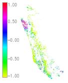
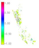
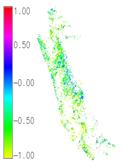
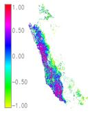
These trends gave an overall idea of the expected relationship between vegetation and climatic variables and motivated us to explore these covariates on a pixel by pixel basis for each year to enhance visualisation of the spatial patterns and on an image to image basis for better numerical description with the time-series monthly data as discussed below. Figure 37–45 shows pixel to pixel correlation maps between NDVI, LST and rainfall for the northern, central and southern Western Ghats from 2003 to 2012.
2003
2004
2005
2006
2007
2008
2009
2010
2011
2012
Figure 37: Pixel to pixel correlation maps between NDVI and LST for northern Western Ghats.
2003
2004
2005
2006
2007
2008
2009
2010
2011
2012
Figure 38: Pixel to pixel correlation maps between NDVI and rainfall for northern Western Ghats.
2003
2004
2005
2006
2007
2008
2009
2010
2011
2012
Figure 39: Pixel to pixel correlation maps between LST and rainfall for northern Western Ghats.
2003
2004
2005
2006
2007
2008
2009
2010
2011
2012
Figure 40: Pixel to pixel correlation maps between NDVI and LST for central Western Ghats.
2003
2004
2005
2006
2007
2008
2009
2010
2011
2012
Figure 41: Pixel to pixel correlation maps between NDVI and rainfall for central Western Ghats.
2003
2004
2005
2006
2007
2008
2009
2010
2011
2012
Figure 42: Pixel to pixel correlation maps between LST and rainfall for central Western Ghats.
2003
2004
2005
2006
2007
2008
2009
2010
2011
2012
Figure 43: Pixel to pixel correlation maps between NDVI and LST for southern Western Ghats.
2003
2004
2005
2006
2007
2008
2009
2010
2011
2012
Figure 44: Pixel to pixel correlation maps between NDVI and rainfall for southern Western Ghats.
2003
2004
2005
2006
2007
2008
2009
2010
2011
2012
Figure 45: Pixel to pixel correlation maps between LST and rainfall for southern Western Ghats.
NDVI and LST were negatively correlated (at 99% confidence interval) in most areas during 2003 to 2012 in northern and central Western Ghats (figure 37 and 40) reestablishing that vegetation and dense forest decrease surface temperature. Northern Western Ghats showed minimum positive correlation value of 0.96 in 2009 and 2011 and a minimum negative correlation of -0.99 in 2011–2012 and central Western Ghats had minimum positive correlation value of 0.95 in 2012 and a minimum negative correlation of -0.99 in 2007, 2008, and 2010–12. However, a similar observation was not noticed in southern Western Ghats (figure 43) where weak negative to strong positive correlation was found during 2004–2008 and 2010 suggesting the possible effects of temperature on NDVI in most parts of the region (with a maximum positive correlation value of 0.99 in 2003-4 and a minimum negative correlation of -0.95 in 2004). The positive correlation may have been caused due to high temperature even with dense vegetation as this region has equatorial climatic influence which enhances photosynthesis and respiration for plant growth (Mao et al., 2012). In contrast, 2003, 2009, 2011–12 showed negative correlation.
Rainfall is the most important source of soil moisture; NDVI was closely linked with rainfall. Most areas showed weak negative to strong positive correlation (figure 38) between NDVI and rainfall during 2003–2012; the year 2009 exhibited very high correlation in the entire region. This reaffirmed that forest tend to bring rainfall in tropical region. The minimum positive and negative correlation was 0.93 in 2004 and -0.96 in 2009. A strip of area stretched from the center to the southernmost part of the image representing water body on the ground (with negative NDVI values) showed negative correlation whereas LST and rainfall showed positive correlation in this area. For the central Western Ghats, from 2003 to 2008, weak negative to positive correlation was found in most of the region except southern most part, where correlation was strongly positive. From 2009 to 2012, weak negative to strong positive correlation was observed stretching from the center to eastern most part of the region from north to south (figure 41) with a minimum positive correlation of 0.95 in 2007 and 2011 and a minimum negative correlation of -0.93 in 2006. In southern Western Ghats, 2003 to 2008 exhibited stronger negative to weak positive correlation whereas, the trend changed to weak negative to stronger positive correlation from 2009–12 (figure 44) with a minimum positive correlation of 0.88 in 2008 and minimum negative correlation of -0.97 during 2005–6 and 2009–12.
Increasing temperature enhances the intensity of transpiration, and decreasing precipitation reduces the available moisture for plants (Yang et al., 2009). The relationship between LST and rainfall in the northern Western Ghats had many variations for each year. Only data of 2003 showed positive relationship whereas 2004 and 2007 depicted positive correlation in northern part and negative correlation in southern half of the region (2004 data seems to have image anomaly). All other years showed negative to weak positive correlation with a minimum positive correlation value of 0.46 in 2006 and a minimum negative correlation value of -0.31 in 2003 in the region with weak positive correlation mainly corresponding to water bodies (figure 39). Data of central Western Ghats showed both weak negative to strong positive correlation for the year 2003–5, 2007, 2009, 20011–12. The remaining years show stronger positive correlation. The minimum positive correlation was 0.74 in 2004 to a minimum of -0.66 in 2007 (figure 42). Southern Western Ghats region showed weak negative to positive correlation in the year 2003–4 and strong negative correlation in 2009 and 2012. Stronger positive correlation exist for the year 2005–8, 2010–11 with a minimum positive correlation of 0.87 in 2003 and a minimum negative correlation of -0.17 in 2005 (figure 45).
To further understand the relationship between NDVI and climatic variables, image to image correlation coefficient (CC or r) values between monthly NDVI of forest with LST and rainfall, and monthly NDVI of agriculture/grassland class with LST and rainfall for northern, central and southern Western Ghats were computed. Table 9–11 shows monthly correlation values of 2003 and 2012 for forest and agriculture class. For other years, correlation tables are provided in Appendix 2. Correlation between monthly LST and rainfall were not computed as they did not reveal any information in previous analysis and their pattern were not clear. Missing data have been shown with "--". The analysis reconfirmed the negative correlation between NDVI and LST in northern and central Western Ghats and negative to weak positive correlation in southern Western Ghats. Most months showed weak negative to strong positive correlation between NDVI and rainfall during 2003–2012 in northern and central Western Ghats. Southern Western Ghats exhibited stronger negative to weak positive correlation between 2003 to 2008 and weak negative to stronger positive correlation from 2009–12 between NDVI and rainfall further corroborating the pixel to pixel analysis. In northern and central region, at the beginning of the summer months, most of the trees (apart from the evergreen forest) have limited vegetation growth, hence strong negative correlation implies increased temperature in those areas and less precipitation. The situation prevails until monsoon arrives at the end of summer season.
Table 9: Image to image Pearson product-moment correlation coefficient (CC or r) between monthly NDVI of forest and agriculture/grassland class with LST and rainfall for northern Western Ghats
Month, Year
CC (r) (NDVI-LST)
CC (r) (NDVI-rainfall)
Month, Year
CC (r) (NDVI-LST)
CC (r) (NDVI-rainfall)
Forest
Jan, 2003
--
-0.09
Jan, 2012
-0.41
-0.16
Feb, 2003
--
-0.06
Feb, 2012
-0.54
-0.13
Mar, 2003
-0.65
0.06
Mar, 2012
-0.66
-0.15
Apr, 2003
-0.65
0.3
Apr, 2012
-0.73
0.26
May, 2003
-0.63
-0.19
May, 2012
-0.74
0.28
Jun, 2003
-0.43
-0.12
Jun, 2012
-0.24
0.18
Aug, 2003
-0.17
0.09
Aug, 2012
-0.1
0.08
Sep. 2003
-0.36
-0.05
Sep. 2012
-0.28
0.24
Oct, 2003
-0.73
-0.19
Oct, 2012
-0.65
0.44
Nov, 2003
-0.5
-0.13
Nov, 2012
-0.60
0.08
Dec, 2003
-0.42
0.17
Dec, 2012
-0.41
0.09
Agriculture/grassland
Jan, 2003
--
-0.21
Jan, 2012
-0.47
-0.26
Feb, 2003
--
-0.14
Feb, 2012
-0.5
-0.21
Mar, 2003
-0.41
-0.23
Mar, 2012
-0.34
-0.16
Apr, 2003
-0.38
-0.05
Apr, 2012
-0.23
-0.14
May, 2003
-0.31
-0.15
May, 2012
-0.26
-0.18
Jun, 2003
-0.18
0.27
Jun, 2012
-0.16
0.15
Aug, 2003
-0.1
-0.03
Aug, 2012
-0.22
0.17
Sep. 2003
-0.39
0.33
Sep. 2012
-0.16
0.08
Oct, 2003
-0.55
0.38
Oct, 2012
-0.22
0.01
Nov, 2003
-0.67
-0.26
Nov, 2012
-0.49
-0.1
Dec, 2003
-0.55
0.11
Dec, 2012
-0.54
-0.1
Table 10: Image to image Pearson product-moment correlation coefficient (CC or r) between monthly NDVI of forest and agriculture/grassland class with LST and rainfall for central Western Ghats
Month, Year
CC (r) (NDVI-LST)
CC (r) (NDVI-rainfall)
Month, Year
CC (r) (NDVI-LST)
CC (r) (NDVI-rainfall)
Forest
Jan, 2003
--
-0.24
Jan, 2012
-0.24
0.0
Feb, 2003
--
-0.31
Feb, 2012
-0.21
0.07
Mar, 2003
-0.7
-0.2
Mar, 2012
-0.26
0.27
Apr, 2003
-0.78
-0.06
Apr, 2012
-0.29
0.29
May, 2003
-0.75
-0.15
May, 2012
-0.07
0.38
Jun, 2003
-0.29
0.26
Jun, 2012
-0.10
0
Aug, 2003
-0.07
0.16
Aug, 2012
-0.4
-0.03
Sep. 2003
-0.55
0.24
Sep. 2012
-0.05
-0.04
Oct, 2003
-0.60
-0.05
Oct, 2012
0.02
-0.11
Nov, 2003
-0.65
0.27
Nov, 2012
-0.34
0.36
Dec, 2003
-0.61
0.05
Dec, 2012
-0.42
0.20
Agriculture/grassland
Jan, 2003
--
0.04
Jan, 2012
-0.44
0.1
Feb, 2003
--
0.13
Feb, 2012
-0.27
0.2
Mar, 2003
-0.21
0.18
Mar, 2012
-0.24
0.3
Apr, 2003
-0.21
0.26
Apr, 2012
-0.21
0.3
May, 2003
-0.17
-0.01
May, 2012
-0.15
0.4
Jun, 2003
-0.45
0.23
Jun, 2012
-0.26
0.16
Aug, 2003
-0.06
0.12
Aug, 2012
0.08
0.06
Sep. 2003
-0.08
-0.08
Sep. 2012
-0.2
0.04
Oct, 2003
-0.48
0.37
Oct, 2012
-0.4
0.21
Nov, 2003
-0.39
0.35
Nov, 2012
-0.31
0.32
Dec, 2003
-0.41
0.03
Dec, 2012
-0.3
0.1
Table 11: Image to image Pearson product-moment correlation coefficient (CC or r) between monthly NDVI of forest and agriculture/grassland class with LST and rainfall for southern Western Ghats
Month, Year
CC (r) (NDVI-LST)
CC (r) (NDVI-rainfall)
Month, Year
CC (r) (NDVI-LST)
CC (r) (NDVI-rainfall)
Forest
Jan, 2003
--
-0.06
Jan, 2012
-0.58
0.16
Feb, 2003
--
0.17
Feb, 2012
-0.68
0.2
Mar, 2003
-0.42
-0.06
Mar, 2012
-0.58
0.15
Apr, 2003
-0.66
-0.55
Apr, 2012
-0.47
0.5
May, 2003
-0.19
0.41
May, 2012
-0.17
0.33
Jun, 2003
-0.28
-0.09
Jun, 2012
-0.43
0.23
Aug, 2003
-0.18
-0.07
Aug, 2012
-0.18
0.00
Sep. 2003
-0.38
0.11
Sep. 2012
-0.32
0.19
Oct, 2003
-0.24
0.22
Oct, 2012
-0.05
0.24
Nov, 2003
-0.42
0.16
Nov, 2012
-0.73
-0.04
Dec, 2003
-0.58
-0.13
Dec, 2012
-0.62
-0.21
Agriculture/grassland
Jan, 2003
--
0.13
Jan, 2012
0.00
0.00
Feb, 2003
--
-0.25
Feb, 2012
0.00
0.03
Mar, 2003
-0.08
0.17
Mar, 2012
0.24
-0.09
Apr, 2003
0.00
-0.02
Apr, 2012
0.32
0.28
May, 2003
0.19
-0.15
May, 2012
0.13
0.24
Jun, 2003
0.23
0.1
Jun, 2012
0.37
-0.16
Aug, 2003
0.07
0.04
Aug, 2012
0.41
0.15
Sep. 2003
-0.43
0.06
Sep. 2012
0.15
0.26
Oct, 2003
-0.36
0.11
Oct, 2012
0.22
0.08
Nov, 2003
0.33
0.01
Nov, 2012
0.26
-0.05
Dec, 2003
-0.11
-0.02
Dec, 2012
-0.11
0.1
Through long-term data analysis, trends in ecological indicators can also be assessed (Orr et al., 2004). The ultimate goal of the time-series analysis of the historical biophysical data is to improve our forecasting capability and make inferences about climate and drought conditions while improving critical vegetation mapping capabilities associated with critical needs such as production estimates, habitat assessments, etc.
It is critical to understand the responses of dense vegetation growth to environmental change and to get a better understanding of the interactions between terrestrial ecosystem and climatic parameters.
The magnitude of the seasonal NDVI and its change over time are important indicators of the contribution of vegetation activity in different seasons to total annual plant growth (Piao et al., 2003). Western Ghats is characterised by three main seasons namely, summer (which spans from March to May), monsoon (June to October), and winter (November to February). Seasonal NDVI for summer, monsoon and winter were computed that is the average monthly composite NDVI for the three seasons. To detect the variation trends in NDVI with climatic variables (LST and rainfall) for each season (Zhang et al., 2013), a least-square regression was applied as follows:
During monsoon, negative relationship between vegetation and temperature was keenly observed in northern and central Western Ghats and a weak positive correlation in southern Western Ghats. Vegetation also had a negative correlation with rainfall in all the three regions. Vegetation was more negatively correlated with rainfall than with temperature.
In winter season, northern and southern Western Ghats experienced a positive correlation between vegetation and temperature and a weak negative correlation was found in central region. Rainfall was strongly positively correlated with vegetation in northern region and negatively correlated in central and southern Western Ghats. Thus whether temperature and rainfall were the main climate factors affecting vegetation productivity varied with region, season and TP. In southern Western Ghats, NDVI were alternatively regulated by temperature and rainfall in different seasons (see table 15, southern Western Ghats column). However, monsoon and winter NDVI was more correlated with temperature than with rainfall, with similar results been reported by Mao et al., (2012). The overall decline in vegetation may be attributed to decreasing rainfall and low soil temperature that do not provide suitable environment for growth of vegetation.
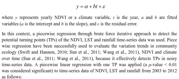
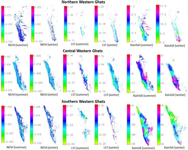
though the trends in seasonal NDVI were complicated and exhibited variations, a high degree of spatial heterogeneity on per-pixel analysis was found. Figure 52 shows spatial patters of the summer and winter seasons NDVI trend for dense vegetation class and table 16 gives the numerical description of the rate of change. Monsoon trend images were not generated as the data had presence of cloud.
Table 16: Rate of change of forest NDVI, LST and rainfall for summer and winter season
Northern Western Ghats
NDVI (yr-1)
LST (°C yr-1)
rainfall (mm yr-1)
Rate of change
ha
%
Rate of change
ha
%
Rate of change
ha
%
Summer
-0.034 – 0
545690
21.17
-0.071 – 0
381750.23
81.98
-4.7 – 0
2394457
93.26
0 – 0.031
2032031
78.83
0 – 0.067
83902.52
18.02
0 – 1.2
173056
6.74
Winter
-0.020 – 0 0
120106.98
18.58
-1.28 – 0
735611.38
97.92
8 – 20
389266
13.19
0 – 0.022
526321.77
81.42
0 – 0.92
15593.07
2.08
20 – 37
2562328
86.81
Central Western Ghats
NDVI (yr-1)
LST (°C yr-1)
rainfall (mm yr-1)
Rate of change
ha
%
Rate of change
ha
%
Rate of change
ha
%
Summer
-0.034 – 0
458812
27.72
-0.82 – 0
1604316
88.98
5.2 – 10
138067.26
19.66
0 – 0.051
1196283
72.28
0 – 0.41
198623
11.02
10 – 21.2
564167.96
80.34
Winter
-0.022 – 0
427804
16.15
-0.74 – 0
2223262
72.66
-35 – -10
4323886
97.64
0 – 0.032
2221605
83.85
0 – 0.76
836761
27.34
-10 – -6
104338
2.36
Southern Western Ghats
NDVI (yr-1)
LST (°C yr-1)
rainfall (mm yr-1)
Rate of change
ha
%
Rate of change
ha
%
Rate of change
ha
%
Summer
-0.045 – 0
1282187
31.79
-0.04 – 0
473.76
0.06
-26 – 0
4067942
86.73
0 – 0.046
2750969
68.21
0 – 0.51
754192.03
99.94
0 – 9
622483
13.27
Winter
-0.029 – 0
737212
30.62
-0.25 – 0
20790
1.95
18 – 30
882285
31.8
0 – 0.028
1670660
69.38
0 – 0.51
1046397
98.05
30 – 74
1892024
68.2
Figure 52: Spatial distribution of trends (rate of change) in summer and winter season for forest NDVI (yr-1), LST (°C yr-1) and rainfall (mm yr-1).
A positive rate of change in NDVI (0-0.031 yr-1) in almost 78.83% of the south-western part of northern Western Ghats was observed in summer. In the same region, a downward trend (-0.2 to -4.7 mm yr-1) was observed in rainfall in the summer months in 93% of the area. The pixels that showed moderate increasing trends in NDVI were mainly distributed in the western part of central Western Ghats (0 to 0.051 yr-1) in 72% of the area in summer and (0 to 0.032 yr-1) in winter season in nearly 84% of the area. Central Western Ghats also exhibited 0.3 to 0.1 °C yr-1 in summer (see figure 52: LST (summer) in central western Ghats) and -0.3 to 0.3 °C yr-1 in winter. The rainfall trend varied with a wide range in both summer and winter. In southern Western Ghats, the NDVI rate of change ranged between -0.015 to 0.02 and -0.01 to 0.01 yr-1 in > 70% of the area in summer and winter (see figure 52). LST data had many missing pixels and did not reveal much information. Rainfall varied with a wide range with maximum change happening at -6 mm yr-1 in summer and 74 mm yr-1 in winter in the southern-most part of the southern Western Ghats.
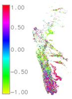
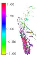
Figure 53–55 shows pixel to pixel correlation between NDVI of forest and LST, and NDVI of forest and rainfall in summer, monsoon and winter for the three regions of Western Ghats. Summer season showed positive correlation between NDVI–LST and NDVI–rainfall in south-western region in 2003 which showed a decreasing pattern in 2012. In monsoon season, correlation between NDVI–LST was not evident because of lack of data and NDVI–rainfall showed weak positive correlation in both 2003 and 2012. Winter depicted a similar pattern in 2003 and 2012 where correlation between NDVI–LST and NDVI–rainfall did not indicate much change in the decade. NDVI–LST showed low and weak negative correlation and NDVI–rainfall showed high positive correlation between 0.5 towards 0.75 (figure 53).
Summer
2003
2012
NDVI-LST
NDVI-rainfall
NDVI-LST
NDVI-rainfall
Monsoon
NDVI-LST
NDVI-rainfall
NDVI-LST
NDVI-rainfall
Winter
NDVI-LST
NDVI-rainfall
NDVI-LST
NDVI-rainfall
Figure 53: Pixel to pixel correlation between forest NDVI, LST and rainfall for summer, monsoon and winter season for northern Western Ghats.
Summer
2003
2012
NDVI-LST
NDVI-rainfall
NDVI-LST
NDVI-rainfall
Monsoon
NDVI-LST
NDVI-rainfall
NDVI-LST
NDVI-rainfall
Winter
NDVI-LST
NDVI-rainfall
NDVI-LST
NDVI-rainfall
Figure 54: Pixel to pixel correlation between forest NDVI, LST and rainfall for summer, monsoon and winter season for central Western Ghats.
One of the challenges posed by climate change is ascertainment, identification and quantification of trends in rainfall to assist in formulation of adaptation and mitigation measures through appropriate strategies of water resource management (Kampata et al., 2008). Rainfall is one of the key climatic variables that affects spatio-temporal patterns on water availability (De Luis et al., 2000). Therefore, analysis of rainfall trends is important to understand the impacts of climate change for water resource management (Haigh, 2004).
Non-stationary rainfall data in modelling hydrological systems often produce erroneous water resource scenarios (IPCC, 2007). Analysis of trends in rainfall is both temporal and spatial in dimension, so the trends of temporal time-series need to be analysed for homogeneity within the region. An attempt is made here to see if the decadal rainfall pattern in the individual three regions of Western Ghats belong to similar regime, have had any significant trends and if there was a homogeneity in trends among stations. The objective is to determine any intervention on the rainfall time-series and subsequently study the trends in the non-intervened series of monthly rainfall. For this, data from rain gauge stations in the northern, central and southern Western Ghats were used. Rainfall data are sometimes exposed to step or gradual changes (Ndiritu, 2005) due to anthropogenic or natural factors which bring inconsistencies and non-homogeneity in the data. Therefore, data from the individual rain gauge stations need to be assessed for intervention analysis before the trend analysis to confirm if data from individual rainfall stations belong to the same population or climatic regime as explained in the steps below:
Intervention analysis – This was carried out using CUSUM (cumulative summation) technique (Parida et al., 2003) to determine inconsistencies in rainfall data which might have resulted from climate change and/or anthropogenic activities. CUSUM is based on the cumulative sum of the data. If X1, X2, ..., Xn represents n data points, then cumulative sum (Si) is for i = 1 to n. The cumulative sum is the cumulative sum of differences between the values and the average . Since the average is subtracted from each value, the cumulative sum ends at zero i.e. Sn = 0. When the series under test is free from any intervention, the plot of Si versus i normally oscillates around the horizontal axis. A steady decline or rise of this plot suggests the possibility of intervention from the year of observation. Positive slopes indicate a period of above average values of rainfall and a negative slope indicates vice versa. The two series may split by the date of change due to possible intervention and require step change analysis for confirmation of the change.
Step change analysis – Wilcoxon-Mann-Whitney rank-sum test (Helsel and Hirsch, 2002) is a nonparametric test used for testing the difference in median of two subsets of data representing the before and after-event/intervention to analyse any step change. Rank-sum test overcomes the problem of small sample sizes and distribution (Yue et al., 2002). The data are first ranked from smallest to largest and in case of ties (equal data values), the average of rank is used. Next, sum of the ranks of the observations in the smaller group and in the larger group are computed along with the mean and standard deviation of the entire sample. The null hypothesis H0 is that no change has occurred in the time-series or the two samples come from the same population (i.e. have the same median) is accepted when the computed statistic is less than the value obtained from a normal distribution table at a specific significance level.
Trend analysis – Trend analysis is carried using Mann-Kendall method which is a non-parametric test and can be used to analyse trends of rainfall (Burns et al., 2007; Ndiritu, 2005). A positive value of the test statistic indicates an increasing trend and a negative value indicates a decreasing trend. The null hypothesis H0 is that there is no trend in the data which is either accepted or rejected depending on the value of the test statistic at a specified significance level.
Test of homogeneity of stations – This is used by combining data from several stations to obtain a single global trend (Helsel and Hirsch, 2002) through Mann-Kendall statistic for each rain gauge station. To test the homogeneity of trends at multiple stations, the homogeneity statistic is calculated. The null hypothesis H0 is that the stations are homogeneous with respect to the trend, and is tested by comparing to tables of distribution with p-1 degrees of freedom, where "p" is the number of rain gauge stations. If it exceeds the critical value for the preselected '' then H0 is rejected and conclusions are made that different stations exhibit different trends.
10 rain gauge stations were selected in northern, 11 in central and 19 in southern Western Ghats. For each station, monthly rainfall data were collected from 2003 to 2012. Intervention analysis, step change analysis, trend analysis and test of homogeneity were carried out for each station. We present here analysis of 2 random locations from each region. For northern region, CUSUM plots of Mumbai and Goa are shown in figure 56. Figure 57 shows the CUSUM plots for Honavar and Udupi in central, and figure 58 shows CUSUM plots for Kozhikode and Thiruvananthapuram in southern Western Ghats. The monthly rainfall time-series from figure 56 clearly show that for most of the periods the monthly rainfall have been below the long-term mean with an intervention in May, 2005 in northern Western Ghats. For central Western Ghats, Honavar and Udupi shows oscillating patterns with increasing trends in the later part of the decade as shown in figure 57. These two stations (Honavar and Udupi) indicate May, 2007 as the year of intervention. Figure 58 indicates a decreasing pattern with below long-term mean values, and increasing pattern with above long-term mean values in the second half of the decade in southern Western Ghats. Some intervention is seen during April, 2004 in the data.
Figure 56: CUSUM plots using observed monthly total rainfall for Mumbai and Goa (January, 2003 to December, 2012). Figure 57: CUSUM plots using observed monthly total rainfall for Honavar and Udupi (January, 2003 to December, 2012). Figure 58: CUSUM plots using observed monthly total rainfall for Kozhikode and Thiruvananthapuram (January, 2003 to December, 2012).
However, to confirm the intervention, the data were subjected to step change analysis. The null hypothesis and alternate hypothesis are stated as below:
H0 = No change has occurred in the time-series.
H1 = Change has occurred in the time-series.
At a 0.05 significance level, Wilcoxon-Mann-Whitney rank-sum test showed different results as indicated in table 17.
Table 17: Results of step change analysis using rank sum method
Rain gauge station
Test statistic W
p-value
Result
Mumbai
1330
0.4329
Not significant, Accept H0
Goa
909
0.0015
Significant, Reject H0
Honavar
783.5
0.1287
Not significant, Accept H0
Udupi
1549
0.2286
Not significant, Accept H0
Kozikode
355
0.0002
Significant, Reject H0
Thiruvananthapuram
479
0.0064
Significant, Reject H0
Mumbai data showed that there was no strong evidence against H0, hence H0 was accepted and there was no intervention, while for Goa data, H0 was rejected in favour of H1 indicating an intervention. In central Western Ghats, Honavar and Udupi did not show any change in regime while in the southern Western Ghats, Kozikode and Thiruvananthapuram data showed signs of interventions and revealed that annual rainfall time-series did not belong to the same population.
The trends for each station were investigated using the Mann-Kendall test. The null hypothesis and alternate hypothesis are:
H0 = There is no trend in the data.
H1 = There is trend in the data.
At a 0.05 significance level, Mann-Kendall test showed the following results as indicated in table 18.
Table 18: Trend analysis using Mann-Kendall method
Rain gauge station
Kendall's tau statistic
2-sided p-value
Result
Mumbai
-0.0136
0.83717
Not significant Accept H0
Goa
0.126
0.051248
Not significant Accept H0
Honavar
0.0435
0.54447
Not significant Accept H0
Udupi
0.0362
0.56683
Not significant Accept H0
Kozikode
0.0926
0.13785
Not significant Accept H0
Thiruvananthapuram
0.0491
0.42853
Not significant Accept H0
For all the stations, there was no evidence of significant trends (due to lack of strong evidence against H0 ), therefore, no trends were observed in Mumbai, Goa, Honavar, Udupi, Kozikode and Thiruvananthapuram rainfall data as the computed statistic were found to be less than the critical value at . Rainfall showed a very small increasing trend except in Mumbai, where a small decreasing trend was observed.
For a region wise analysis about the trend at multiple rain gauge stations, the test for homogeneity was applied. It is necessary to investigate whether the monthly rainfall data are serially correlated or not through autocorrelation and partial autocorrelation plots corresponding to the time-series data. In case the monthly data are serially correlated, Mann-Kendall test in conjunction with block bootstrapping can be used to account for the correlation. In this study, it was found that the autocorrelation and partial autocorrelation present in the series were not significant. Using the results from Mann-Kendall calculations from table 18, the homogeneity statistic was calculated (Helsel and Hirsch, 2002).
The null hypothesis and alternate hypothesis are:
H0 = Rain gauge stations are homogeneous with respect to trend.
H1 = Rain gauge stations are not homogeneous with respect to trend.
Since was less than the critical value at for all the three regions with p-1 degrees of freedom (where "p" is the number of rain gauge stations in each region), it was concluded that there were no sufficient evidence against H0, so the individual stations in northern, central and southern Western Ghats had homogeneous trends. Modelling and forecasting the monthly rainfall time-series: Understanding and predicting rainfall variability helps in planning and decision making process. Analysis of the time-series data is a very powerful tool to reveal the patterns of data and an important aspect is to find a suitable time-series seasonal model for forecasting the amount of rainfall. The analysis is done with two objectives (Harris and Solis, 2003):
Build a model that fits the data or represents the data well (to find patterns).
Use the model to forecast.
While the analysis is being carried, we assume the data to follow some pattern along with some outliers (random noise). The data can be smoothened using either moving average or median smoothing or exponential smoothing to remove the outliers or random variations. The method of smoothing is chosen on the basis of data and the level of smoothing required. Moving average is simplest but it does not work well with the data having many outliers, in such cases, median smoothing is more useful. Exponential smoothing is believed to be superior since recent observations in the data are given relatively more weightage in forecasting than the older observations. Most time-series patterns can be described in terms of two basic classes of components: trend and seasonality (Brockwell and Davis, 2002).
Trend analysis: Trend is defined as the long term movement in a time-series without calendar related and irregular effects, and is a reflection of the underlying level. It is the result of influences, for example, population growth, general economic changes, etc. There are no proven automatic techniques to identify trend components in the time-series data. More often, trend is visible from the time-series plots which is usually monotonous in nature, either downward or upward. Time-series data can contain trends which may be either linear or exponential or mixed. If the time-series data contain considerable outliers, then the first step in the process of trend identification is smoothing. In this process, the non-systematic components of individual observations cancel out each other hence making the data free of outliers. They filter out the noise and convert the data into a smooth curve that is relatively unbiased by outliers (Harris and Solis, 2003).
Seasonality: A seasonal pattern exists when a series is influenced by seasonal factors (e.g., the quarter of the year, the month, or day of the week). Seasonality is always of a fixed and known period, therefore, seasonal time-series are also called periodic time-series and represents the repetitive component (Harris and Solis, 2003). A cyclic pattern exists when data exhibit trough and crest that are not of fixed period i.e. if the fluctuations are not of fixed period then they are cyclic; if the period is unchanging and associated with some aspect of the calendar, then the pattern is seasonal. In general, the average length of cycles is longer than the length of a seasonal pattern, and the magnitude of cycles tend to be more variable than the magnitude of seasonal patterns. In short, trend represents long-term change in the level of the series, seasonal factor is the periodic fluctuations of constant length and the random part is the error which is unpredictable in behaviour.
A seasonal time-series consists of a trend component, a seasonal component and an irregular component as its constituents. It assumes the following decomposition model:
So, at any time period 't', the mathematical model for decomposing seasonal data can be approximated as
where,
Yt = time-series value (actual data) at period t.
St = seasonal component at period t.
Tt = trend component at period t.
Et = irregular component at period t.
Therefore, decomposing a seasonal time-series means separating the time-series into these three components, i.e., estimating these three components. However, the exact functional form of the time-series data depends on the type of decomposition model as briefed below:
Additive model – An additive model is appropriate if the magnitude of the seasonal fluctuation does not vary with the level of the series.
Multiplicative model – A multiplicative model is more prevalent with economic series since most seasonal economic series have seasonal variations which increases with the level of the series.
Once the time-series is decomposed, a model can be constructed to analyse and forecast the time-series data. In this study we adopt autoregressive integrated moving average (ARIMA) (Brockwell and Davis, 2002), which is one of the most widely used models in analysing and forecasting time-series data. ARIMA models are defined for stationary time-series, therefore, if the data are non-stationary time-series i.e. when the mean and variance of the data points is not constant over a period of time, the time-series is differenced to obtain a stationary series. ARIMA is then fitted to determine whether AR (Auto Regressive) or MA (Moving Average) terms are needed to correct any autocorrelation that remains in the differenced series. By analysing the autocorrelation function (ACF) and partial autocorrelation function (PACF) plots of the differenced series, the numbers of AR and/or MA terms that are needed can be determined. ACF plot is a bar chart of the coefficients of correlation between a time-series and lags of itself and PACF plot is a plot of the partial correlation coefficients between the series and lags of itself. From this, an ARIMA(p, d, q) model is obtained, where "p" is the value of autocorrelation for the time-series or auto-regression part, "d" is the order of differencing used or trend part and "q" is the partial autocorrelation for the time-series or the moving average part.
Auto-regressive component (p) – These components represent the memory of the process of previous observations. p in ARIMA(p, d, q) refers to number of auto-regressive components. If it is 1, then the current observation is correlated with its previous observation. If its value is 2, then the observations are correlated with the observations at lag 2.
Trend component (d) – When time-series data have trend component, then the mean and variance are not constant over time, so it is differentiated once to make the mean constant and d in ARIMA(p, d, q) is set to 1 else the time-series data are differentiated again to make the mean constant and d is set to 2. Differencing is the easiest way to make a non-stationary time-series into stationary time-series. The residual plot and the Normal Q-Q (normal quantile-quantile) plot are generally linear. The Box-Pierce test is used to check the significance of normality of the residual at a specified lag.
Moving-averages component (q)– These components represent the memory of the process for previous random shocks, i.e., random components in the time-series. q refers to number of auto-regressive components in the ARIMA(p, d, q). If it is 1, then the current observation is correlated with the random shock at lag 1. If its value is 2, then the observations are correlated with the random shocks at lag 2.
ARIMA model includes an explicit statistical model for the irregular component of a time-series that allows non-zero autocorrelations in the irregular component. This feature is not supported by exponential smoothing method, therefore ARIMA model is preferred for forecasting. In this study, the seasonal rainfall time-series is assumed to be of the additive model form since the random fluctuations in the data are roughly constant over time and do not depend on the level of time-series i.e. there is a seasonal variation in the amount of rainfall per month. Adf (Augented Dickey-Fuller test) and the pp test (Phillips-Perron Unit Root test) were performed to check for the stationarity. The Dickey-Fuller Z(alpha) was -5.1208, Truncation lag parameter was 1 and p-value was 0.000821 indicating that the null hypothesis H0: data is stationary was true.
Figure 59 shows the rainfall time-series plot of forest cover for northern, central and southern Western Ghats, all of them highlighting a seasonal component. Figure 60 shows the decomposition of additive time-series into original time-series (top), the estimated trend component (second from top), the estimated seasonal component (third from top), and the irregular component (bottom). The highest seasonal factor is observed in July and August and the lowest is recorded from December through April for each year in northern Western Ghats. The estimated seasonal component shows increasing trend in rainfall from May to August and a decreasing trend from September to April in this region. In central and southern Western Ghats, highest seasonal factor is seen in June and lowest is observed in January–February. Here, the estimated seasonal component shows increasing trend in rainfall from April to June and a decreasing trend from July to March.
Figure 59: Rainfall time-series plots over dense forest cover.
Figure 60: Decomposition of time-series – observed, trend, seasonal and random components over dense forest cover.
ARIMA(0,0,1) was found to be most suitable for northern, and ARIMA(1,0,0) with non-zero mean was adapted for rainfall data pertaining to central and southern Western Ghats. These models were used to make forecasts for future values of the rainfall time-series. Figure 61 shows the forecast plots for the three regions from 2013 to 2020 in blue line, 80% prediction interval as dark grey shaded area, and 95% prediction interval as light grey shaded area. Appendix 3(table 1–3)details the monthly forecasted rainfall values from 2013 to 2020 for the forest class for northern, central and southern Western Ghats.
Figure 61: Time-series forecast plots of rainfall over forest cover for the northern, central and southern Western Ghats.
Figure 62 shows the rainfall time-series plots over agriculture/grassland areas for northern, central and southern Western Ghats highlighting a seasonal component. Figure 63 shows decomposition of additive time-series into original (top), estimated trend component, estimated seasonal component, and the irregular component (bottom). The highest and the lowest seasonal factor of rainfall in agriculture/grassland LC was similar to that of forest LC type (i.e. high in July and August and low from December to April) in northern Western Ghats. The estimated seasonal component also showed increasing trend in rainfall from May to August and a decreasing trend from September to April. Even the central and southern Western Ghats indicated similar trends of rainfall in agriculture/grassland areas as that of forest cover i.e. highest seasonal factor was seen in June and lowest was observed in January–February. The estimated seasonal component also showed increasing trend in rainfall from April to June and a decreasing trend from July to March.
Figure 62: Rainfall time-series plots over agriculture/grassland land cover.
Figure 63: Decomposition of time-series – observed, trend, seasonal and random components of rainfall in agriculture/grassland land cover.
Figure 64: Time-series forecast plots of rainfall in agriculture/grassland areas for the northern, central and southern Western Ghats.
ARIMA(0,0,1) was used for forecasting the rainfall pattern in agricultural/grassland areas in northern Western Ghats, and ARIMA(1,0,0) with non-zero mean was used for rainfall data pertaining to central and southern Western Ghats. Figure 64 shows the forecast plots for the three regions from 2013 to 2020 in blue line, 80% prediction interval as dark grey shaded area, and 95% prediction interval as light grey shaded area. Appendix 3(table 4–6) details the monthly forecasted rainfall values from 2013 to 2020 in the agricultural/grassland areas for northern, central and southern Western Ghats. In general, we see a decreasing trend in the rainfall pattern over vegetative areas (forest and agricultural/grassland) from 2013 towards 2020 in northern, central and southern Western Ghats.
T.V. Ramachandra
Centre for Sustainable Technologies, Centre for infrastructure, Sustainable Transportation and Urban Planning (CiSTUP), Energy & Wetlands Research Group, Centre for Ecological Sciences, Indian Institute of Science, Bangalore – 560 012, INDIA. E-mail : cestvr@ces.iisc.ac.in Tel:91-080-22933099/23600985, Fax:91-080-23601428/23600085 Web:http://ces.iisc.ac.in/energy
Uttam Kumar
Energy and Wetlands Research Group, Centre for Ecological Sciences. Indian Institute of Science, Bangalore – 560 012, India
E-mail: uttam@ces.iisc.ac.in
Anindita Dasgupta Energy and Wetlands Research Group, Centre for Ecological Sciences. Indian Institute of Science, Bangalore – 560 012, India
Bharath Setturu Energy and Wetlands Research Group, Centre for Ecological Sciences. Indian Institute of Science, Bangalore – 560 012, India
E-mail: settur@ces.iisc.ac.in
Vinay S Energy and Wetlands Research Group, Centre for Ecological Sciences. Indian Institute of Science, Bangalore – 560 012, India
E-mail: vinay@ces.iisc.ac.in
Harish R Bhat Energy and Wetlands Research Group, Centre for Ecological Sciences. Indian Institute of Science, Bangalore – 560 012, India
E-mail: harishrbhat@ces.iisc.ac.in
Citation: Ramachandra T V, Uttam Kumar and Anindita Dasgupta, 2016, Time-series MODIS NDVI based Vegetation Change Analysis with Land Surface Temperature and Rainfall in Western Ghats, India, ENVIS Technical Report 100, Sahyadri Conservation Series 53, Energy & Wetlands Research Group, CES, Indian Institute of Science, Bangalore 560012.
Contact Address :
Dr. T.V. Ramachandra
Energy & Wetlands Research Group,
Centre for Ecological Sciences, Indian Institute of Science, Bangalore – 560 012, INDIA. Tel : 91-80-23600985 / 22932506 / 22933099 Fax : 91-80-23601428 / 23600085 / 23600683[CES-TVR] E-mail : cestvr@ces.iisc.ac.in, energy@ces.iisc.ac.in, Web : http://wgbis.ces.iisc.ac.in/energy


 (a) January, 2003
 (b) December, 2012
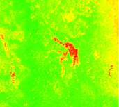
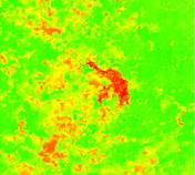
 January, 2003
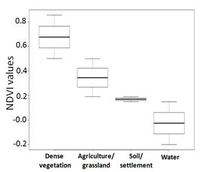 December, 2012
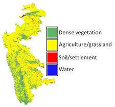


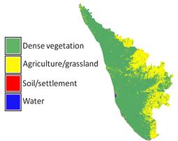
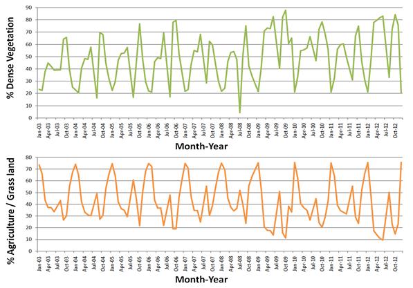


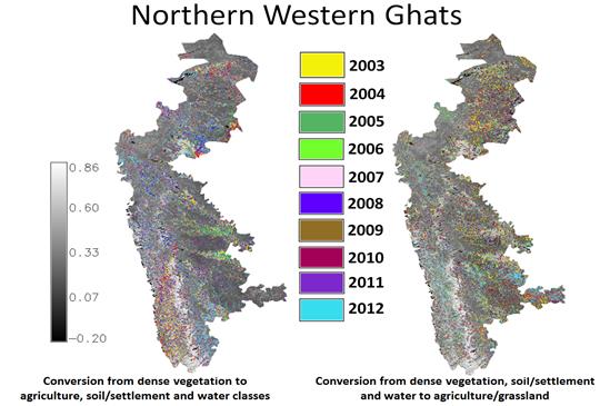
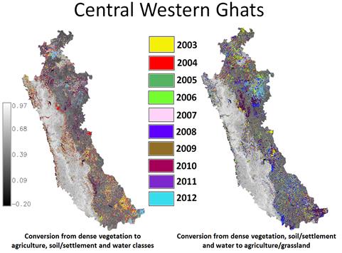
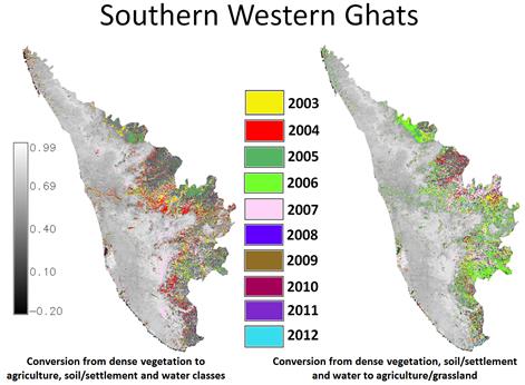
 Dense vegetation (2003)
 Dense vegetation (2012)
 Agriculture/grassland (2003)
 Agriculture/grassland (2012)
 Soil/settlement (2003)
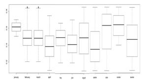 Soil/settlement (2012)
 Water (2003)
 Water (2012)
 Dense vegetation (2003)
 Dense vegetation (2012)
 Agriculture/grassland (2003)
 Agriculture/grassland (2012)
 Soil/settlement (2003)
 Soil/settlement (2012)
 Water (2003)
 Water (2012)
 Dense vegetation (2003)
 Dense vegetation (2012)
 Agriculture/grassland (2003)
 Agriculture/grassland (2012)
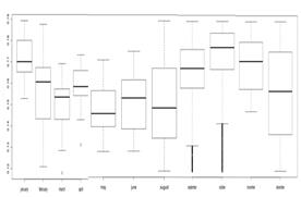 Soil/settlement(2003)
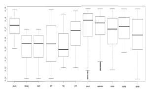 Soil/settlement (2012)
 Water (2003)
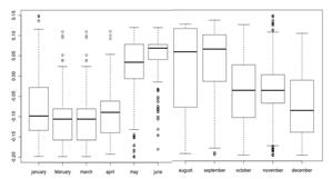 Water (2012)
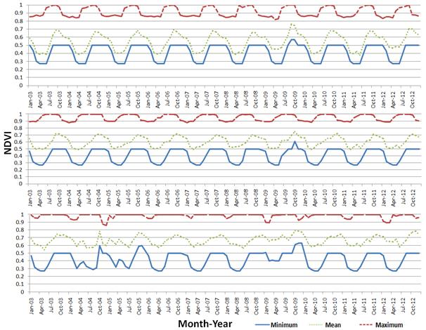
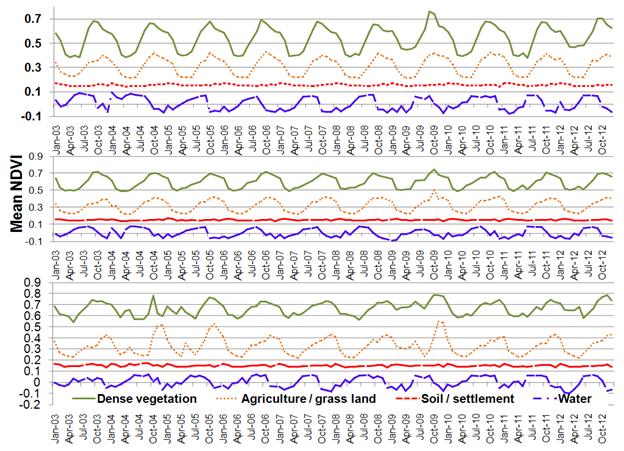
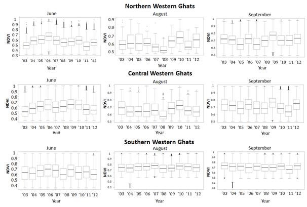

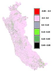
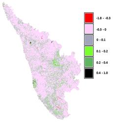
 January, 2003
 February, 2003
 March, 2003
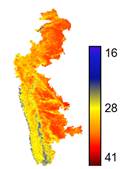 April, 2003
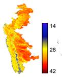 May, 2003
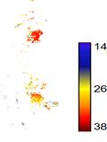 June, 2003
 August, 2003
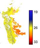 September, 2003
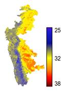 October, 2003
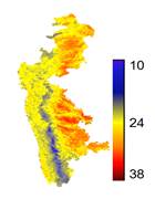 November, 2003
 December, 2003
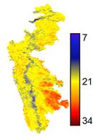 January, 2012
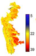 February, 2012
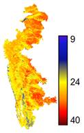 March, 2012
 April, 2012
 May, 2012
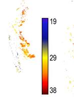 June, 2012
 August, 2012
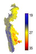 September, 2012
 October, 2012
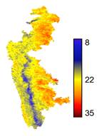 November, 2012
 December, 2012
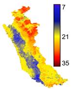 January, 2003
 February, 2003
 March, 2003
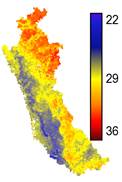 April, 2003
 May, 2003
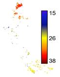 June, 2003
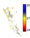 August, 2003
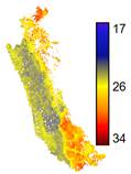 September, 2003
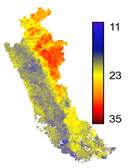 October, 2003
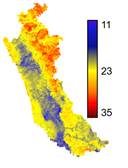 November, 2003
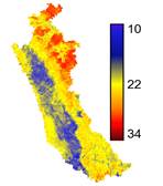 December, 2003
 January, 2012
 February, 2012
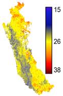 March, 2012
 April, 2012
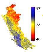 May, 2012
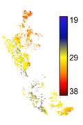 June, 2012
 August, 2012
 September, 2012
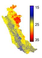 October, 2012
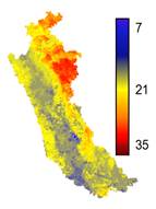 November, 2012
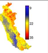 December, 2012
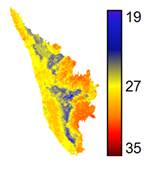 January, 2003
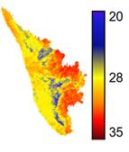 February, 2003
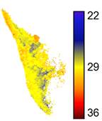 March, 2003
 April, 2003
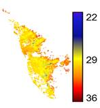 May, 2003
 June, 2003
 August, 2003
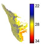 September, 2003
 October, 2003
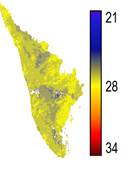 November, 2003
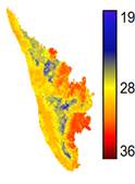 January, 2012
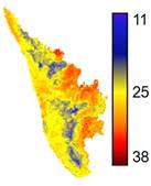 February, 2012
 March, 2012
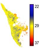 April, 2012
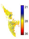
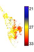 June, 2012
 August, 2012
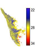 September, 2012
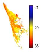 October, 2012
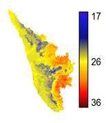 November, 2012
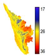 December, 2012
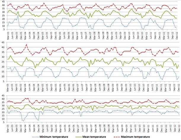
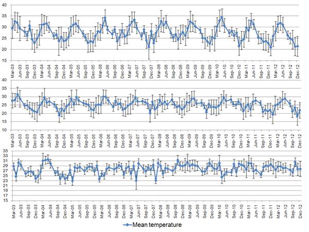
 January, 2003
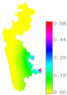 February, 2003
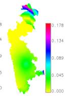 March, 2003
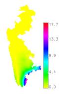 April, 2003
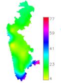 May, 2003
 June, 2003
 July, 2003
 August, 2003
 September, 2003
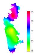 October, 2003
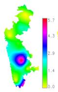 November, 2003
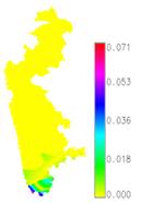 December, 2003
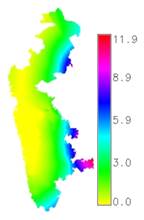 January, 2012
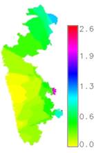 February, 2012
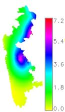 March, 2012
 April, 2012
 May, 2012
 June, 2012
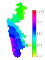
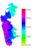 August, 2012
 September, 2012
 October, 2012
 November, 2012
 December, 2012
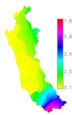 January, 2003
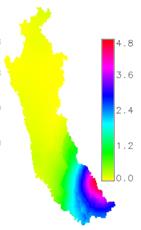 February, 2003
 March, 2003
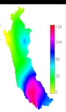 April, 2003
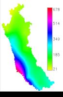 May, 2003
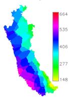 June, 2003
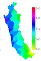 July, 2003
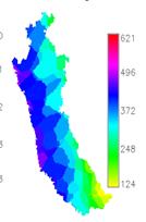 August, 2003
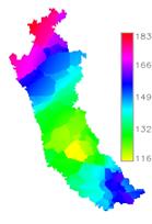 September, 2003
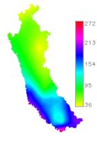 October, 2003
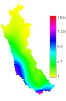 November, 2003
 December, 2003
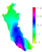 January, 2012
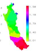 February, 2012
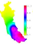 March, 2012
 April, 2012
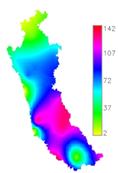
 June, 2012
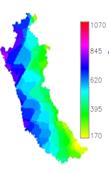 July, 2012
 August, 2012
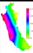 September, 2012
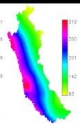
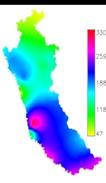 November, 2012
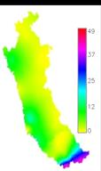
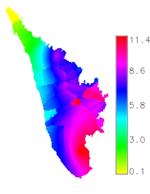 January, 2003
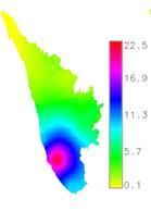 February, 2003
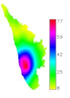 March, 2003
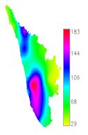 April, 2003
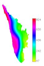 May, 2003
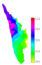 June, 2003
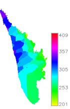 July, 2003
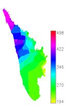 August, 2003
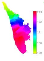 September, 2003
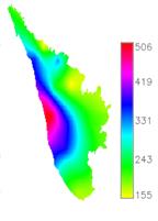 October, 2003
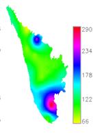 November, 2003
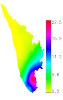 December, 2003
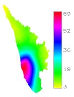 January, 2012
 February, 2012
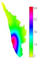 March, 2012
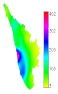 April, 2012
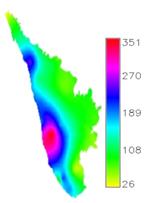 May, 2012
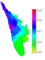 June, 2012
 July, 2012
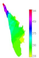 August, 2012
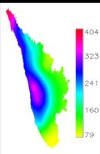 September, 2012
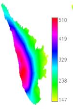 October, 2012
 November, 2012
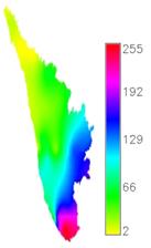 December, 2012
 2003
2003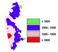 2004
2004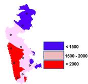 2005
2005 2006
2006 2007
2007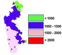 2008
2008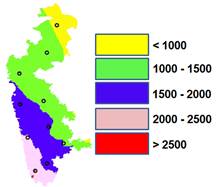 2009
2009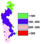 2010
2010 2011
2011 2012
2012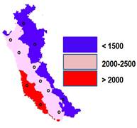 2003
2003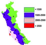 2004
2004 2005
2005 2006
2006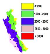 2007
2007 2008
2008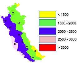 2009
2009 2010
2010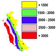 2011
2011 2012
2012 2003
2003 2004
2004 2005
2005 2006
2006 2007
2007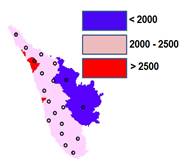 2008
2008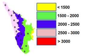 2009
2009 2010
2010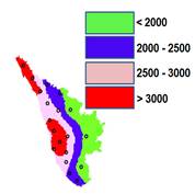 2011
2011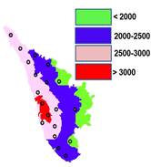 2012
2012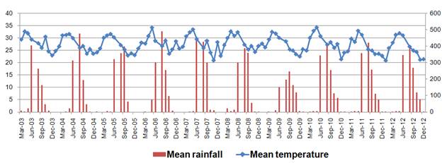
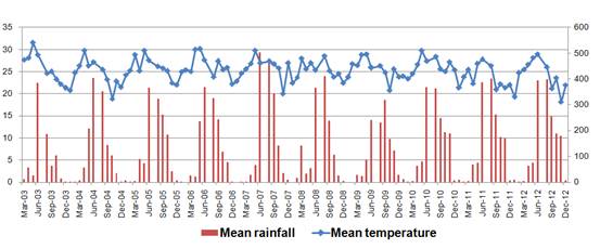

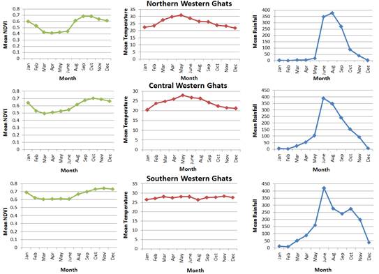

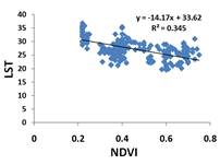
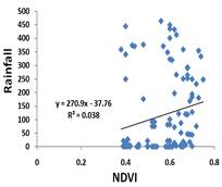
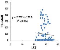

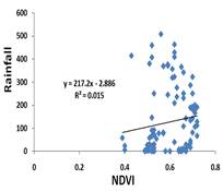
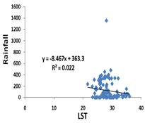

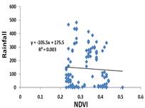

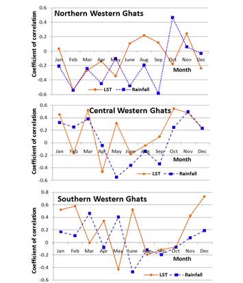
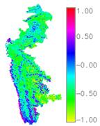 2003
2003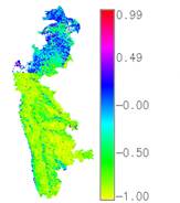 2004
2004 2005
2005 2006
2006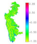 2007
2007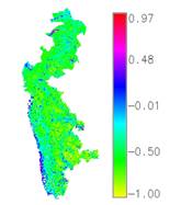 2008
2008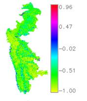 2009
2009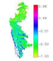 2010
2010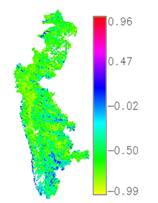 2011
2011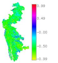 2012
2012 2003
2003 2004
2004 2005
2005 2006
2006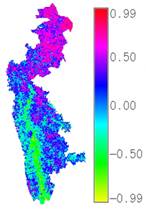 2007
2007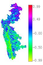 2008
2008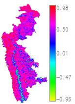 2009
2009 2010
2010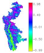 2011
2011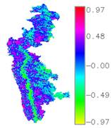 2012
2012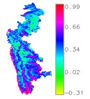 2003
2003 2004
2004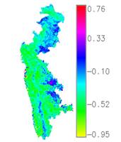 2005
2005 2006
2006 2007
2007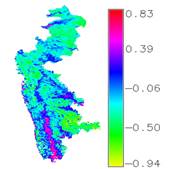 2008
2008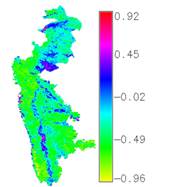 2009
2009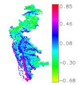 2010
2010 2011
2011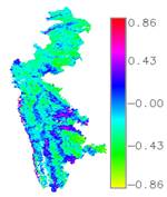 2012
2012 2003
2003 2004
2004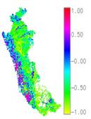 2005
2005 2006
2006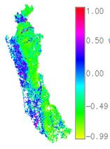 2007
2007 2008
2008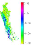 2009
2009 2010
2010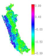 2011
2011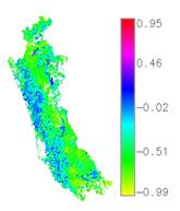 2012
2012 2003
2003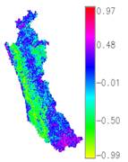 2004
2004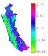 2005
2005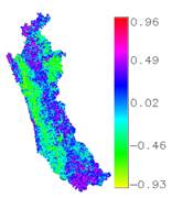 2006
2006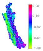 2007
2007 2008
2008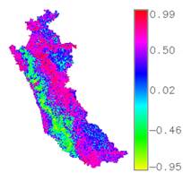 2009
2009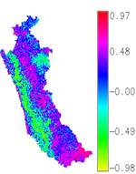 2010
2010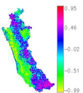 2011
2011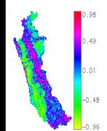 2012
2012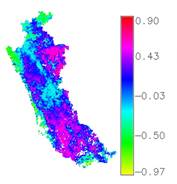 2003
2003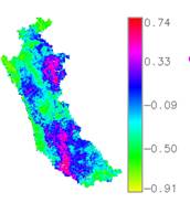 2004
2004 2005
2005 2006
2006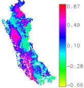 2007
2007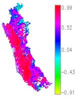 2008
2008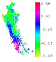 2009
2009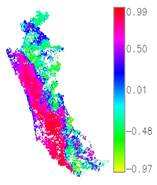 2010
2010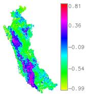 2011
2011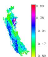 2012
2012 2003
2003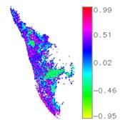 2004
2004 2005
2005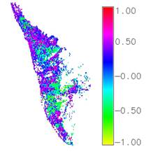 2006
2006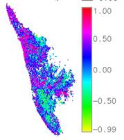 2007
2007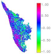 2008
2008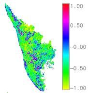 2009
2009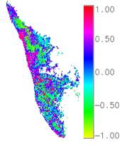 2010
2010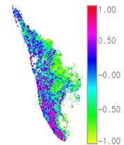 2011
2011 2012
2012 2003
2003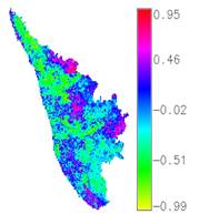 2004
2004 2005
2005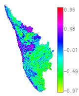 2006
2006 2007
2007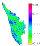 2008
2008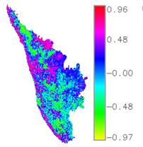 2009
2009 2010
2010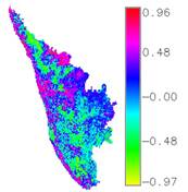 2011
2011 2012
2012 2003
2003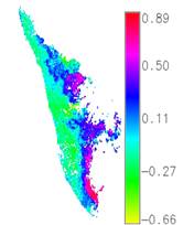 2004
2004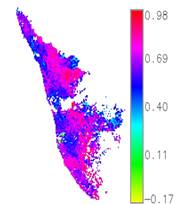 2005
2005 2006
2006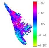 2007
2007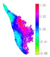 2008
2008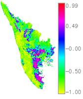 2009
2009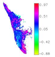 2010
2010 2011
2011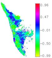 2012
2012