Uttam Kumar [uttam@ces.iisc.ernet.in]

Norman Kerle [kerle@itc.nl]

Milap Punia [m_punia@hotmail.com]

T. V. Ramachandra* [cestvr@ces.iisc.ernet.in]

Results

Classification of LISS-III

The class spectral characteristics for 6 LC categories using LISS-III MSS band 2, 3 and 4 were obtained from the training pixels spectra to assess their inter-class separability and the images were classified as shown in Figure 4 (A) with training data collected using pre-calibrated GPS, uniformly distributed over the study area. This was validated with the representative field data and the LC statistics are given in Table 1. Producer’s, User’s, and Overall accuracy computed are listed in Table 2. A kappa (k) value of 0.95 was obtained, indicating that the classified outputs are in good agreement with the ground conditions to the extent of 95%. The possible source of errors in classification was mainly due to the temporal difference in training data collection (December, 2005) and image acquisition (December, 2002).

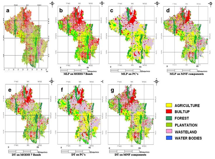
Fig. 4 Classified images of LISS-III (a), MLP on MODIS 7 bands (b), MLP on PCs of MODIS 36 bands (c), MLP on MNF components of MODIS 36 bands (d), DT on MODIS 7 bands (e), DT on PCs of MODIS 36 bands (f), DT on MNF components of MODIS 36 bands (g)

Table 1. Land Cover details from LISS-III MSS and MODIS

Classes %	LISSIII	7 Bands		PCs		MNF
		NN	DT	NN	DT	NN	DT
Agriculture	19.0	21.9	18.0	21.5	22.1	19.4	21.7
Built up	17.1	26.4	16.4	15.8	16.0	17.6	17.6
Forest	11.4	07.7	13.1	12.0	09.6	11.3	10.2
Plantation	11.0	19.3	11.5	09.5	11.4	10.8	09.4
Waste land	40.4	24.4	40.2	40.3	38.3	40.0	40.4
Water	01.1	00.3	00.7	00.9	02.6	00.9	00.8

Table 2. Accuracy of LC classification using ground truth

Land use	Agriculture		Built up		Forest		Plantation		Waste land		Water bodies		Overall Accuracy
Accuracy Algorithm	U*	P*	U	P	U	P	U	P	U	P	U	P
MLC (LISSIII)	94	85	97	83	95	96	92	92	98	90	96	98	95.63
NN (B1 to B7)	98	70	95	93	89	73	59	97	71	77	48	69	71.89
NN (PCA)	64	41	79	81	75	82	69	83	63	72	63	74	70.10
NN (MNF)	94	58	81	99	95	87	86	99	74	95	89	57	86.11
DT (B1 to B7)	74	57	98	93	81	94	63	45	94	90	59	37	71.02
DT (PCA)	63	52	62	80	68	86	61	36	66	53	46	23	68.88
DT (MNF)	74	50	95	92	89	91	95	93	74	93	55	37	74.66

                 *U – User’s accuracy, P – Producer’s accuracy. Highest figures are marked in bold.

The same data was also classified in 1000 iterations using NN where the training threshold contribution was set to 0.1, training rate was 0.2, training RMSE was 0.09, number of hidden layers was 1 and the output activation threshold was 0.001. The overall accuracy was 95.1% with producer’s and user’s accuracy in the range of 85-96% and 85-95% respectively, and a kappa (k) value of 0.94.

Even though the outputs obtained from MLC and NN were very close to each other in terms of overall accuracy (95.63% for MLC and 95.1% for NN), MLC output was marginally superior and was used as a reference to validate the output of the MODIS products. Choice of MLC was more justified, as the time complexity involved in training the neurons in NN was very high compared to MLC and NN classification became more complex with the large image size of LISS-III MSS (5997 rows x 6142 columns). This conventional per-pixel spectral-based classifier (MLC) constitutes a historically dominant approach to RS-based automated land-use/land-cover (LULC) derivation (Gao et al., 2004; Hester et al., 2008) and in fact, this aids as “benchmark” for evaluating the performance of novel classification algorithms (Song et al., 2005). The dimension of MODIS data was very less (532 rows x 546 columns) and hence it is reasonable to rigorously apply and choose appropriate classification algorithm. In this context, we applied MLC, NN and DT on different products of MODIS, but used MLC based LISS-III MS classified map for evaluating the MODIS outputs.

Classification of MODIS

The MODIS data (bands 1 to 7), the first five PC’s and the first five MNF components of the MODIS 36 bands (based on their higher eigen values) were classified using MLP [Figure 4 (B), (C), (D)]. The order of presentation of training samples was randomized from epoch to epoch and the momentum and learning rate parameters were adjusted as the number of training iterations increased. The process for training the neurons converged at 1000 iterations. The number of hidden layer was kept at 1, the output activation function and momentum were kept low and increased in steps to see the variations in the classification result. The RMS error at the completion of the process was 0.09, 0.39 and 0.29 for the three different inputs, respectively. Figure 5 shows the training iterations on the three different data sets. DT-See5 was used to classify the same three datasets. For each training site, a level of confidence in characterization of the site was recorded as described below:

1. The scaled reflectance values for LC classes were extracted for all the ground points.
2. All the data were converted into See5 compatible format and was submitted for extraction of rules.
3. Since the boosting option changes the exact confidence of the rule, the rules were extracted without boosting option. A 10% cut off was allowed for pruning the wrong observations.
4. Once the rules were framed by the See5, these rules were ported into Knowledge engineer to make a knowledge based classification schema. It was ensured that 90% confidence level is maintained for all the classes defined.
5. Subsequently the decision tree schema was applied over the data set to produce the colour coded land cover output [Figure 4 (E), (F), (G)].

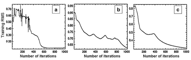
Fig. 5. Training RMS vs. Iterations for (A) MODIS 7 bands, (B) PCs of MODIS 36 bands and (C) MNF components of MODIS 36 bands

Table 3 shows the total number of rules generated, the maximum and the minimum confidence level for each class and the number of rules used for classification at a confidence level of 0.600 for MODIS 7 band data. For MODIS derived PCs, the rules were generated at a confidence level of 0.920 (table 4). Here the image was classified into more number of classes (16) and these classes were ultimately merged into six categories. For the MNF bands, the threshold factor was maintained at 0.7 at a confidence level 0.700 (table 5). Table 1 shows the LC statistics for the classification results.

Class	Rules generated	Confidence level Maximum               Minimum		Number of Rules Confidence level – 0.600
Agriculture	87	0.982	0.563	60
Built up (Urban/Rural)	27	0.988	0.551	21
Evergreen/ Semi-Evergreen Forest	9	0.958	0.667	6
Plantation/ orchards	85	0.981	0.648	53
Waste land/Barren Rock / Stony waste	43	0.929	0.253	35
Water bodies	17	0.955	0.625	11

 

Class	Rules generated	Confidence level Maximum          Minimum		Number of Rules Confidence level – 0.920
Class 1	49	0.989	0.737	36
Class 2	29	0.997	0.944	20
Class 3	3	0.944	0.833	2
Class 4	2	0.354	0.315	1
Class 5	25	0.985	0.591	11
Class 6	31	0.989	0.800	18
Class 7	31	0.993	0.688	13
Class 8	4	0.875	0.667	1
Class 9	6	0.929	0.800	1
Class 10	2	0.833	0.833	1
Class 11	2	0.929	0.889	1
Class 12	4	0.917	0.875	1
Class 13	2	0.938	0.875	1
Class 14	3	0.963	0.875	1
Class 15	2	0.944	0.833	1
Class 16	3	0.889	0.722	1

 

Class	Rules generated	Confidence level Maximum               Minimum		Number of Rules Confidence level -  0.700
Agriculture	59	0.989	0.500	58
Built up (Urban/Rural)	24	0.996	0.875	25
Evergreen/ Semi-Evergreen Forest	64	0.995	0.971	63
Plantation/ orchards	43	0.970	0.667	44
Waste land/ Barren Rock / Stony waste	36	0.993	0.500	36
Water bodies	5	0.929	0.750	5

Accuracy Assessment

1. Ground truth/field data: User’s, Producer’s and Overall accuracy assessment of the MODIS classified maps was performed with the ground truth data that were collected using handheld GPS in the same month (December, 2005) as that of the RS data acquisition representing the entire study area. 30 test samples were used for validating agriculture, builtup, forest, plantation and waste land classes each and 10 test samples were used for validating water bodies. Survey of India Topographical sheets (1:50000) were also used to validate the results (table 2). The table highlights that some of the LC classes have been classified with higher accuracy using NN while DT has outperformed in classifying the other remaining LC classes. This is explained in detail in the discussion section.    

2. Sub-regional level: At the sub-regional (taluk) level, MODIS based LC class percentages were compared with LISS-III MSS based LC class percentages. The assessment showed that NN analysis of MODIS band 1 to 7 is best for mapping agriculture (with -5% differences between values from LISS-III mapped agriculture), while it fails for plantation and water bodies. DT on MODIS 7 bands is superior for mapping built up (-2.4%), waste land (+1%) and also good for mapping plantation (+2%) with MNF components of 36 bands. While NN on MNF could map forest properly with -3.5% difference and water bodies with +1% difference on sub-region wise distribution. Hence, further analysis was carried out at pixel level to understand the sources of these differences.

3. Pixel level: A pixel of MODIS (250 m) corresponds to a kernel of 10 x 10 pixels of LISS-III spatially (figure 6). Classified maps using MODIS data were validated pixel by pixel with the classified LISS-III image. A kernel of 10 x 10 in LISS-III for a particular category was considered as homogeneous when the presence of that class was ≥ 90%. User’s, Producer’s and Overall accuracy is listed in table 6.

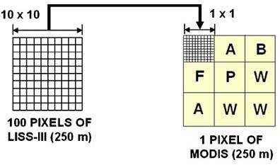
Fig. 6. 10×10 pixels of LISS-III equals to 1×1 pixel of MODIS spatially

Land use	Agriculture		Built up		Forest		Plantation		Waste land		Water bodies		Overall Accuracy
Accuracy Algorithm	U*	P*	U	P	U	P	U	P	U	P	U	P
NN (B1 to B7)	43	59	45	65	61	38	34	59	81	71	37	45	62.38
NN (PCA)	20	61	17	29	49	38	69	69	81	60	56	45	61.40
NN (MNF)	37	46	29	41	64	55	61	69	87	83	65	65	69.87
DT (B1 to B7)	41	51	55	44	59	53	67	67	88	65	55	58	62.22
DT (PCA)	34	41	27	44	49	19	44	41	81	61	29	42	51.34
DT (MNF)	31	31	41	56	61	53	75	76	82	78	48	43	63.69

                  *U – User’s accuracy, P – Producer’s accuracy. Highest figures are marked in bold.

U. Kumar Department of Management Studies and Centre for Sustainable Technologies, Indian Institute of Science, Bangalore 560012, India e-mail: uttam@ces.iisc.ernet.in		M. Punia Centre for the Study of Regional Development, Jawaharlal Nehru University, New Delhi 110067, India e-mail: m_punia@hotmail.com
N. Kerle Department of Earth Systems Analysis, Faculty of Geo-Information Science and Earth Observation, Twente University, P.O. Box. 6, 7500 AA Enschede, The Netherlands e-mail: kerle@itc.nl		T. V. Ramachandra (*) Centre for Ecological Sciences and Centre for Sustainable Technologies, Indian Institute of Science, Bangalore 560012, India phone: 91-80-22933099; fax: 91-80-23601428; e-mail: cestvr@ces.iisc.ernet.in

E-mail   |   Sahyadri   |   ENVIS   |   GRASS   |   Energy   |   CES   |   CST   |   CiSTUP   |   IISc   |   E-mail