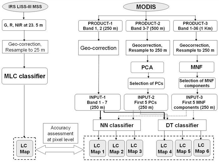
Methods

LISS-III data were geo-corrected, mosaiced, cropped pertaining to study area boundary and resampled to 25 m, (for pixel level comparison with MODIS classified data). Supervised classification was performed using a Maximum Likelihood classifier followed by accuracy assessment. It is to be noted that the same technique did not perform well on coarse resolution data (MODIS) and therefore, we evaluated NN and DT for MODIS data classification. The MODIS data were geo-corrected with an error of 7 m with respect to LISS-III images. The 500 m resolution bands 3 to 7 and 1 km MODIS 36 bands were resampled to 250 m using nearest neighbour (with Polyconic projection and Evrst 1956 as the datum). Principal components (PC) and minimum noise fraction (MNF) components were derived from the 36 bands to reduce noise and computational requirements for subsequent processing. The methodology is depicted in figure 2. The spectral characteristics of the training data were analysed using spectral plots and a Transformed Divergence matrix. MODIS data were classified using MLP and DT. The MLP based NN classifier and DT is briefly discussed below.

Fig. 2 Steps involved in methodology for obtaining LC maps

MLP based NN classifier

 NN classification overcomes the difficulties in conventional digital classification algorithms that use the spectral characteristics of the pixel in deciding to which class a pixel belongs. The bulk of MLP based classification in RS has used multiple layer feed-forward networks that are trained using the back-propagation algorithm based on a recursive learning procedure with a gradient descent search. A detailed introduction can be found in literatures (Atkinson and Tatnall, 1997; Duda et al., 2000; Haykin, 1999; Kavzoglu and Mather, 1999; Kavzoglu and Mather, 2003; Mas, 2003) and case studies (Bischof et al., 1992; Chang and Islam, 2000; Heermann and Khazenie, 1992; Venkatesh and Kumar Raja, 2003).

The MLP in this work is trained using the error backpropagation algorithm (Rumelhart et al., 1986). The main aspects here are: (i) the order of presentation of training samples should be randomised from epoch to epoch; and (ii) the momentum and learning rate parameters are typically adjusted (and usually decreased) as the number of training iterations increases. Back propagation algorithm for training the MLP is briefly stated below:

1. Initialize network parameters: Set all the weights and biases of the network to small random values.
2. Present input and desired outputs: Present a continuous valued input vector, x₀, x₁,…, x_n-1, and specify the desired output d₀, d₁…d_n-1. If the network is used as a classifier, then all the desired outputs are typically set to zero except for that corresponding to the class of the input. That desired output is 1.
3. Forward computation: Let a training example in the epoch be denoted by [x(n), d(n)], with the input vector x(n) applied to the input layer of sensory nodes and the desired response vector d(n) presented to the output layer of computation nodes, The net internal activity v_j^(l)(n) for the neuron j in layer l is given by equation (1)

                                                                                          (1)

   where    is the function signal of neuron i in the previous layer (l-1) at iteration n, and  is the synaptic weight of neuron j in the layer l that is fed from neuron i in layer (l-1). Assuming the use of sigmoid function as the nonlinearity, the function (output) signal of neuron j in layer l is given by equation (2)

                                                                                           (2)

   If neuron j is in the first hidden layer (i.e., l=1), set yj(0) = xj(n), where x_j(n) is the jth element of the input vector x(n). If neuron j is in the output layer (i.e., l=L), set . Hence, compute the error signal , where d_j(n) is the j^th element of the desired response vector d(n).

4. Backward computation: Compute the δ’s (i.e., the local gradients) of the network by proceeding backward, layer by layer:

   , for neuron j in output layer L,

   

   , for neuron j in the hidden layer l.
   Hence adjust the synaptic weights of the network in layer l according to the generalised delta rule (equation 3):

                                                     (3)

   where η is the learning-rate parameter and α is the momentum constant.

5. Iteration: Iterate the forward and backward computations under Steps 3 and 4 by presenting new epochs of training examples to the network until stopping criterion is met.

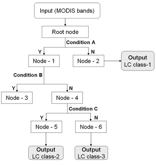
Decision Tree

Decision tree (DT) is a machine learning algorithm and a non-parametric classifier involving a recursive partitioning of the feature space, based on a set of rules learned by an analysis of the training set. A tree structure is developed; a specific decision rule is implemented at each branch, which may involve one or more combinations of the attribute inputs. A new input vector then travels from the root node down through successive branches until it is placed in a specific class (Piramuthu, 2006) as shown in figure 3. The thresholds used for each class decision are chosen using minimum entropy or minimum error measures. It is based on using the minimum number of bits to describe each decision at a node in the tree based on the frequency of each class at the node. With minimum entropy, the stopping criterion is based on the amount of information gained by a rule (the gain ratio). DT algorithm is stated briefly:

Fig. 3 General structure of a data mining decision tree

1. If there are k classes denoted {C₁, C₂,….C_k}, and a training set, T, then
2. If T contains one or more objects which all belong to a single class C_j, then the decision tree is a leaf identifying class C_j.
3. If T contains no objects, the decision tree is a leaf determined from information other than T.
4. If T contains objects that belong to a mixture of classes, then a test is chosen, based on a single attribute that has one or more mutually exclusive outcomes {O₁, O₂,…O_n}. T is portioned into subsets T₁, T₂,…T_n, where T_i contains all the objects in T that have outcome Oi of the chosen test.

The same method is applied recursively to each subset of training objects to build DT. Successful applications of DT using MODIS data have been reported in Chang et al., (2007) and Wardlow and Egbert (2008). Accuracy assessment was done for the classified maps with ground truth data. LC percentages were compared at sub-regional level (taluk level) and at pixel level with a LISS-III classified map.