Cellular automata (CA) growth modeling

This section discusses in detail the design of the CA urban growth modeling. The design phases include: transition rule definition, calibration method and evaluation strategy for the model. Calibration modules for accurate modeling over the historical satellite imagery to adapt the urban pattern.

1.      CA algorithm design

The design of the CA algorithm consists of defining the transition rules that control the urban growth, calibrating these rules, and evaluating the results for prediction purpose as shown in figure 5. Transition rules definition is the most important phase in CA model design since they translate the effect of input data on the urban process simulation. The CA algorithm design starts with defining the transition rules that drive the urban growth over time. They are designed as a function of land use effect on urban process, growth constraints and population density. The transition rules are defined over the 3 x 3 neighbourhood of a pixel to minimize the number of input variables to the model. The rules identify the neighbourhood needed for the tested cell to urbanise.

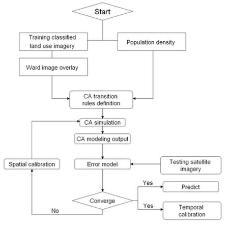
Figure 5: Flowchart of CA algorithm design.

The growth constraints should reflect the conservation strategy adopted in the study area for certain land uses. For example, conservation of certain species of natural resources can be taken into consideration through rules definition stage. Water resources protection through discouraging urban growth nearby these sites to preserve them over time is another example of constrained rules design. The future state of a pixel (Equation 4) at time (t+1) from starting time (t) depends on three factors:

• Current state of the pixel

• Current states of the neighbourhood pixels

• Transition rules that drive the urban growth over time

      
                                                  …..      (Equation 4)

where

 = test pixel future state at time epoch t+1
 = test pixel current state at time epoch t
 = neighbourhood pixels states’ set.

2.       CA Model calibration

Calibration aims to define the best set of CA rules based on which the model runs to match as close as possible to the simulated results with the ground truth images. To achieve this purpose, two calibration schemes are introduced in this algorithm: spatial and temporal calibrations. In spatial calibration module, the CA transition rules at a given time t are modified spatially over the 2D grid space. This is done through tuning the values of each rule set on a directional basis to match the urban dynamics for each township with its site specific features. This allows the model to take the variability in the spatial urban growth pattern into account for realistic modeling. If the CA rules in a direction result in higher growth levels (overestimated), they are modified to reduce the urban growth in that direction. For the underestimation case, the rule values of the direction under consideration are tuned to increase the amount of urban growth to match the real one. So, the spatial calibration aims to find the best set of rule values that fit a given direction according to its geographical location.

The oldest historical classified Landsat MSS image (of 1973) subset for Bangalore city (figure 6) from the Greater Bangalore image (figure 2) is used as input to the CA model over which the transition rules are applied to model the urban growth starting from this time epoch. Dividing the study area on a direction and further on a ward basis will take into consideration the effect of site specific features in each direction on the urban growth. The same CA transition rules are defined for each direction, however, with different rule values. CA transition rules (f) of the developed model were physically built over the input imagery and the rules used a 3 x 3 neighbourhood -  in equation 5 to identify the test pixel future state,  in equation 6.

Figure 5: Bangalore city in 1973, 1992 and 2006 used in the CA model for simulation (subset from Greater Bangalore classified image).

                                                …..      (Equation 5)

                                                                                                   …..      (Equation 6)

Transition rules (f) were designed to identify the required neighborhood urban level for a test pixel to urbanise. The following is a summary of such rules:

• IF test pixel is water, road OR urban (residential or commercial) THEN no change.

• IF test pixel is non-urban (vegetation OR open land) THEN it becomes urban if its:

• Population density is equal or greater than threshold (Pi) AND neighbouring residential pixel count is equal or greater than threshold (Ri)

where (R,C)i are integer numbers ranging from 0 to 8 (3 x 3 neighborhood) and Pi is a real number ranging from 0 to 1 (0.1 increment; population density values were normalized from 0 to 1 for each direction in order to have effective CA rules calibration). The calibration (i.e., identifying best (R,P)i parameter values) of such rules was performed spatially on a ward level, Tw to fit the local urban dynamic features and over  time to consider the temporal urban changes in each direction, Tt in (7).

Ø calibrated = f(Tw, Tt, f)                                                                                     …..      (Equation 7)

f in the calibration formula represents the criteria selected to find the best rule set for certain  ward spatial location Tw at given time epoch Tt. This criterion in our model represents the total modeling errors/mismatch between modeled output and reality that need to be minimised or best match. f in (8) was defined as a function of fitness F in (9) and total errors ∆E in (10) valuation measures. Fitness and total errors measure the compatibility in terms of urban count and pattern within each township with respect to reality, respectively (Al-Kheder, et al., 2007).

                                                                               …..      (Equation 8)

                                                  …..      (Equation 9)

                                                                …..      (Equation 10)

Once the CA transition rules were identified and initialized for each direction, the model runs from 1973 till 1992. The 1992 image represents the first ground truth being used for calibration. For each ward, the modeling accuracy is calculated as a ratio between the simulated and real urban growth data. Over/underestimation concept is introduced to represent how comparable is the simulated result to the real one. This indicates how transition rules defined on a directional basis succeed in modeling the real amount of urban growth given the predefined conditions. Calibration in this work is meant to find the best set of rule values specific to each direction for realistic urban growth modeling.