Data Preparation

This section describes the input data processing scheme. The two types of input data are:

1. classified images of 1973, 1992 and 2006.

2. population density maps for the year 1973 and 1992.

Landsat Multispectral Scanner (MSS) of 1973 (in Blue (B), Green (G), Red (R) and Near Infrared (IR) bands of 79 m spatial resolution), Landsat Thematic Mapper (TM) of 1992 (B, G, R Near IR, Mid IR-1 and Mid IR-2 bands of 30 m spatial resolution), and IRS Linear Imaging Self Scanner (LISS) - III of 2006 (in G, R and NIR bands of 23.5 m spatial resolution) were used for the generation of land use maps. The data are stored in 8-bit format, i.e. each pixel can take any value from 0 to 255 (28 = 256 values). The values of these pixels in the image are called digital numbers which represents the reflectance represented by that pixel corresponding to the same geographical location on the ground. The 1973 image was of size 429 rows x 445 columns, size of 1992 image was 1130 x 1170 and the size of 2006 image was 1445 x 1496. The differences in the size of the images are due to variations in the spatial resolution of the pixels (79 m, 30 m, and 23.5 m). These data were rectified and registered for systematic errors with the known ground control points that were identifiable in the image as well as Survey of India (SOI) topographical sheets of 1:50000 scale and projected to Polyconic system with Geographic Latitude-Longitude coordinate system and Evrest56 as the datum. All data were resampled to 23.5 m spatial resolution having 1445 rows x 1496 columns to fit each other spatially. Six classes of interest were identified from the false colour composite images: residential areas, commercial areas, roads, vegetation, water, and open land.

Supervised classification of the image was performed using the Maximum Likelihood classifier (MLC). MLC has become popular and widespread in remote sensing because of its robustness (Strahler, 1980; Conese and Maselli, 1992; Ediriwickrema and Khorram, 1997; Zheng et al., 2005). MLC assumes that each class in each band can be described by a normal distribution (Bayarsaikhan et al., 2009). For each land use class (residential areas, commercial areas, roads, vegetation, water, and open land) training samples were collected representing approximately 10% of the study area. With these 10% known pixel labels from training data, the aim was to assign labels to all the remaining pixels in the image.

If the training data (collected from the ground cover using handheld GPS - global positioning system) pertaining to land use classes contain n samples and the samples in each land use class are i.i.d (independent and identically distributed) random variables and further if we assume that the spectral classes for an image is represented by ωi, i=1,…, M, where M is the total number of classes, then probability density p(ωi|x) gives the likelihood that the pixel x belongs to class ωi where x is a column vector of the observed digital number (gray values) of the pixels. It describes the pixel as a point in multispectral space (d-dimensional space, where d is the number of remote sensing spectral bands). The maximum likelihood (ML) parameters are estimated from representative i.i.d samples. Classification is performed according to

                                                         (1)

i.e., the pixel x belongs to class ωi if p(ωi|x) is the largest. The ML decision rule is based on a normalized (Gaussian) estimate of the probability density function of each class. The discriminant function for MLC is expressed as

                                                                                             (2)

where gli(x) stands for the discriminant function for ωi, p(ωi) is the prior probability of ωi, p(x|ωi) is the p.d.f. for pixel vector x conditioned on ωi  (Zheng et al., 2005). Pixel vector x is assigned to the class for which gli(x) is greatest. In an operational context, the logarithm form of (2) is used, and after the constants are eliminated, the discriminant function for ωi is stated as

                                          (3)

where  is the variance-covariance matrix of ωi, Mi is the mean vector of ωi. A pixel is assigned to the class with the lowest  (Zheng et al., 2005; John and Xiuping, 1999, Duda, Hart and Stork, 2001).

Residential, commercial and roads were grouped into a single class – ‘urban’. Final classified images had four land use classes – builtup, vegetation, water and open land (others). The classified images of 1973, 1992 and 2006 had overall accuracies of 72%, 75%, and 73%. Classification was done using the open source programs (i.gensig, i.class and i.maxlik) of Geographic Resources Analysis Support System (http://wgbis.ces.iisc.ernet.in/grass) as displayed in figure 2. The classified images were also verified with field visits and Google Earth image. The class statistics is given in table 1.

Table 1: Greater Bangalore land use statistics

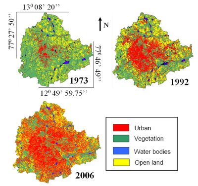
Figure 2: Greater Bangalore in 1973, 1992 and 2006.

Population density is used as the second input for the CA model algorithm. Population census maps for year 1971, 1991 and 2001 over Bangalore city were prepared from the census data. The population densities were computed for all 100 wards by dividing their populations by the ward areas. Figure 3 shows the ward map (left) in each direction and the density for each ward census (right) in 1971, 1991 and 2001. To model the population, the centroid (Xc, Yc) for each ward is calculated.

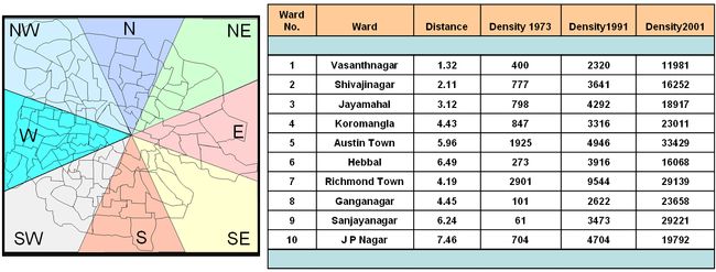
Figure 3: Ward map in each direction and their population densities. Distances are expressed in kilometers and population densities are expressed in persons/sq. km.

The Euclidean distance from each ward centroid to the city center (see figure 1) was computed. This process was repeated for all wards so that a table of population densities versus distance is prepared. Population densities for wards within specified distance from city center were averaged to reduce the variability in data. For example, an average population density for all wards within 0-1 km was calculated, then another average density is calculated for wards within 1-2, 2-3, 3-4 km and so forth. Curves were fitted representing population density as a function of distance from the city centre as shown in figure 4.

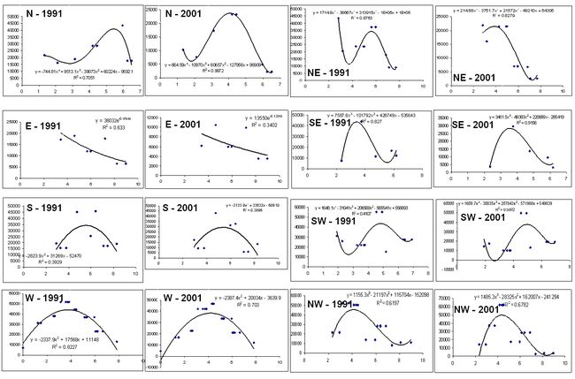
Figure 4: Direction wise population density for the year 1991 and 2001.

The unknown model parameters were calculated for the year 1991 and 2001. These models were used to calculate the population density for each pixel in the imagery based on its distance from the city centre for the year 1991 and 2001. The changes in model parameters over the 10 years (from 1991 to 2001) were used to calculate the yearly rate of change in model parameters. The updated parameters that changed year by year were used to calculate the population density grids for the year 1973 and 1992 matching the same size of the input imagery (remote sensing classified maps - 1445 rows x 1496 columns). These grids were used as the second CA data input for the purpose of running the model over historical growth period.