Methods

Openmodeller, a free and opensource software was used to model landslide occurrence locations. The model utilizes major contributors for landslides like precipitation and six site factors including aspect, DEM, flow accumulation, flow direction, slope, land cover, compound topographic index and historical landslide occurrence points. Precipitation in the wettest month and precipitation in the wettest quarter of the year were considered separately to analyse the effect of rainfall on hill slope failure for generating scenarios to predict landslides.

Genetic Algorithm for Rule-set Prediction (GARP): This is based on genetic algorithms^23,25 and has been widely used for predicting biological species^55,56. GARP develops predictive models consisting of a set of conditional rules in the form of ‘if–then’ statements that describe the ‘niches’ of landslide occurrence points.

GARP uses a set of point localities where the landslide is known to have occurred along with a set of geographic layers representing the environmental parameters that might limit the landslide existence. Genetic Algorithms (GAs) are suitable for solving complex optimization problems and for applications that require adaptive problem-solving strategies. It maps strings of numbers to each potential solution and then each string becomes a representation of individual locations. Then the most promising in its search is manipulated for improved solution⁴⁵. The GARP model is composed of a set of rules developed through evolutionary refinement, testing and selecting rules on random subsets of training data sets. Application of a rule set is more complicated as the prediction system must choose appropriate rule among a number of applicable rules. GARP maximizes the significance and predictive accuracy of rules without over-fitting.

Significance is established through a χ² test on the difference in the probability of the predicted value before and after application of the rule. GARP uses envelope rules, GARP rules, atomic and logit rules. In envelope rule, the conjunction of ranges for all of the variables is a climatic envelope or profile, indicating geographical regions where the climate is suitable for that entity, enclosing values for each parameter. A GARP rule is similar to an envelope rule, except that variables can be irrelevant. An irrelevant variable is one where points may fall within the whole range. An atomic rule is a conjunction of categories or single values of some variables. Logit rules are an adaptation of logistic regression models to rules. A logistic regression is a form of regression equation where the output is transformed into a probability.⁵⁶

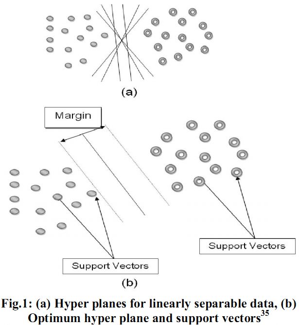
Support Vector Machine (SVM): SVM are supervised learning algorithms based on heuristic algorithms of statistical learning theory²⁷. SVM map input vectors to a higher dimensional space with maximal separating hyper plane. Two parallel hyper planes are constructed on each side of the hyper plane that separates the data. The separating hyper plane maximizes the distance between the two parallel hyper planes. An assumption is made that the larger is the margin or distance between these parallel hyper planes, better will be the accuracy of the classifier. The model produced by support vector classification depends only on a subset of the training data, because the cost function for building the model does not take into account training points that lie beyond the margin.²⁷

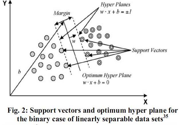
In order to classify n-dimensional data sets, n-1 dimensional hyper plane is produced with SVMs. Fig. 1 illustrates various hyper planes separating two classes of data and there is only one hyper plane that provides maximum margin between the two classes as given in fig. 2 indicating the optimum hyper plane²⁷ and the points that constrain the width of the margin are the support vectors. SVMs locate a hyper plane that maximizes the distance from the members of each class to the optimal hyper plane in the binary case.

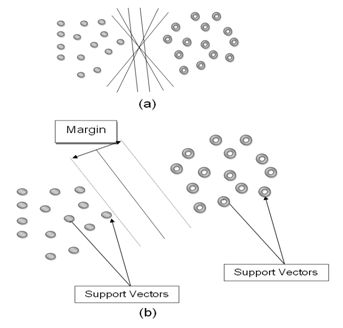
Fig.1: (a) Hyper planes for linearly separable data, (b) Optimum hyper plane and support vectors³⁵

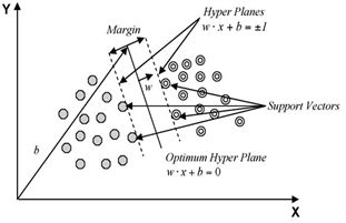
Fig. 2: Support vectors and optimum hyper plane for the binary case of linearly separable data sets³⁵

If there is a training data set containing m number of samples represented by {x_i, y_i} where (i =1, ... , m) x ε RN, N-dimensional space and    y ε {-1, +1} class label and the optimum hyper plane maximizes the margin between the classes. The hyper plane is defined as (w.x_i + b = 0) given in fig. 3, where x is a point lying on the hyper plane, parameter w determines the orientation of the hyper plane in space, b is the bias that the distance of hyper plane from the origin. A separating hyper plane can be defined for two classes for the linearly separable case as:

w . x_i+ b ≥ +1 for all y = +1                                       (1)

w. x_i + b ≤  -1 for all y = -1                                         (2)

These inequalities can be combined into a single inequality:

y_i (w. x_i + b ) – 1 ≥ 0                                                  (3)

The training data points defined by the functions w. x_i+ b = ±1, are the support vectors and lie on these two hyper planes, which are parallel to the optimum hyper plane³⁴. The classes are linearly separable, if a hyper plane exists and satisfies inequality constraints as in (3), with the margin between these planes is equal to 2/||w||³⁴. Thus, the distance to the closest point is 2/||w|| and the optimum separating hyper plane can be found by minimizing ||w||² under the constraint (3).

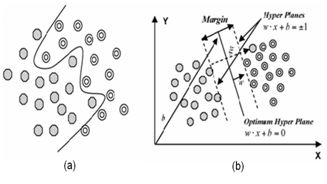
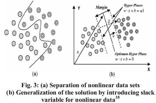
Fig. 3: (a) Separation of nonlinear data sets
(b) Generalization of the solution by introducing slack variable for nonlinear data³⁵

Determination of optimum hyper plane requires solving optimization function is given by:

Min (0.5*||w||² )                                                          (4)
subject to the constraints,

y_i (w. x_i + b ) ≥ -1   and y_i  ε {+1, -1}                          (5)

Fig. 3 (a) illustrates that nonlinearly separable data is the case in various classification problems²⁷ as in the classification of remotely sensed images using pixel samples. In such cases, data sets cannot be classified into two classes with a linear function in input space. The technique can be extended to allow for nonlinear decision surfaces, when it is not possible to have a hyper plane defined by linear equations on the training data.^14,44 Considering this, the optimization problem is replaced by introducing  slack variable [Fig. 3 (b)].

                                                    (6)

subject to constraints,

                     (7)

where C is a penalty parameter or regularization constant . This parameter allows striking a balance between the two competing criteria of margin maximization and error minimization, whereas the slack variables  indicates the distance of the incorrectly classified points from the optimal hyper plane. The larger is the C value, the higher is the penalty associated to misclassified samples.³⁵

Data mapped into a higher dimensional space (H) through nonlinear mapping functions (Ф). An input data point x is represented as Ф(x) in the high-dimensional space. The computation of [Ф(x).Ф(x_i)] is reduced by using a kernel function and  the classification decision function would be: 

                                              (8)

where for each of r training cases there is a vector (x_i) representing the respective spectral response together with a class membership (y_i). α_i (i = 1,….., r) are Lagrange multipliers and K(x, x_i) is the kernel function. The magnitude of α_i is determined by the parameter34 and the kernel function enables the data points to spread in such a way that a linear hyper plane can be fitted¹⁹. The performance of SVMs varies depending on the choice of the kernel function and its parameters. Kernel functions used in SVMs are generally aggregated into four groups namely, linear, polynomial, radial basis function and sigmoid kernels. 

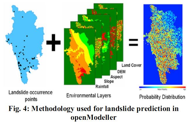
OpenModeller³⁹- a free and open source software was used for predicting the probable landslide areas. OpenModeller (http://openmodeller.sourceforge.net/) is a flexible, user friendly, cross-platform environment and it includes facilities for reading landslide occurrence and environmental data, selection of environmental layers, creating a fundamental landslide prediction model and prediction with various environmental scenarios as shown in fig. 4.

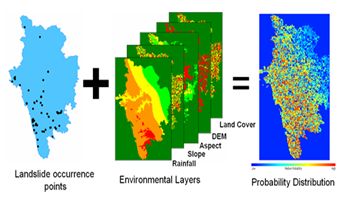
Fig. 4: Methodology used for landslide prediction in openModeller