ABSTRACT

Many shallow landslides are triggered by heavy rainfall on hill slopes resulting in enormous casualties and huge economic losses in mountainous regions. Hill slope failure usually occurs as soil resistance deteriorates in the presence of the acting stress developed due to a number of reasons such as increased soil moisture content, change in land use causing slope instability, etc. Landslides triggered by rainfall can possibly be foreseen in real time by jointly using rainfall intensity-duration and information related to land surface susceptibility. Terrain analysis applications using spatial data such as aspect, slope, flow direction, compound topographic index, etc. along with information derived from remotely sensed data such as land cover / land use maps permit us to quantify and characterise the physical processes governing the landslide occurrence phenomenon. In this work, the probable landslide prone areas are predicted using two different algorithms – GARP (Genetic Algorithm for Rule-set Prediction) and Support Vector Machine (SVM) in a free and open source software package - openModeller. Several environmental layers such as aspect, digital elevation data, flow accumulation, flow direction, slope, land cover, compound topographic index, and precipitation data were used in modelling. A comparison of the simulated outputs, validated by overlaying the actual landslide occurrence points showed 92% accuracy with GARP and 96% accuracy with SVM in predicting landslide prone areas considering precipitation in the wettest month whereas 91% and 94% accuracy were obtained from GARP and SVM considering precipitation in the wettest quarter of the year.           

Index Terms—Landslide, GARP, SVM, openModeller

INTRODUCTION

Landslides are one of the most widespread natural hazards on Earth causing casualties and property loses. They are sudden hydrogeomorphic events due to the combination of i) predisposing factors (e.g. lithology and morphology), ii) triggering factors (e.g. excessive and intense precipitations) and iii) accelerating factors (e.g. human activities altering natural slope stability) [1]. Among landslide typologies, shallow landsliding is common on steep topographies covered by colluvial or residual soils whose texture can vary from sand to clayey silt [2], playing a significant role in hill slope denudation and catchment sediment dynamics. The possible time and locations where landslides are likely to occur should thus be identified in advance in order to avoid or reduce the harm. In this regard, establishing a landslide warning system which provides information for evacuation and hazard mitigating is a top priority.

Prediction of rainfall-triggered hill slope disasters has relied mostly on the valley slope [3 and 4], rainfall intensity and duration that can cause hill slope failure [5, 6, 7 and 8]. Recently, theoretical models have been developed to predict landslide susceptibility based on watershed topographic, geologic and hydrological variables as well as changes in landuse [9, 10, 11, 12, 13 and 14]. The rapidly growing availability of relatively detailed digital elevation data, coupled with simple slope-instability mechanism and hill slope hydrological models, has led to advances in physically-based modeling of shallow landslide hazard [9, 15]. Casadei et al., [16] proposed a landslide warming system using a slope-instability analysis and a hydrological model to predict the time and location of landslides that were verified using historical data of landslide events for Montara Mountains of California from 1953–1998 [17].

Given the complex spatial dynamics of the process, most of the hazard evaluation tools make use of Geographical Information Systems (GIS), capable of geospatial and multitemporal data integration. The availability of digital elevation models (DEMs) and precipitation data at higher spatial and temporal resolution [1] encourage the development of more sophisticated techniques for shallow landslide hazard modelling [9, 15, 18, 19, 20, 21 and 13]. Several of these methods are based on the infinite slope stability equation [22] coupled with hydrological models (e.g. [9, 15 and 13]), extensively applied for the estimation of spatially variable soil wetness (e.g. [23, 24 and 25]). SHALSTAB [9 and 26] is one of these models. Various models have been developed in order to assess landslide incidence potential [27, 28, 29 and 30]. Among these techniques, deterministic, heuristic and statistical methods are the most common ones. Deterministic methods deal with the estimation of quantitative values of stability variables, over a defined area where the landslide types are simple with homogeneous intrinsic properties [31]. The required data include soil strength, depth below the terrain surface, soil layer thickness, slope angle and water pressure. These methods have been employed in translational landslides studies [32] and are applicable at large scale over small areas. One of the main drawbacks of these methods is their high degree of oversimplification when the data are incomplete. Another problem is that the data requirements for deterministic models can be prohibitive, and frequently it is impossible to acquire the input data necessary to use the model effectively.

In this context, the present study explores the suitability of pattern recognition techniques to predict the probable distribution of landslide occurrence points based on several environmental layers along with the known points of occurrence of landslides. The aims of the study are:

1. to apply and evaluate Genetic Algorithm for Rule-set Prediction and Support Vector Machine based models for predicting landslides;
2. to compare and assess the results of these analyses;
3. to suggest management strategies for preventing potential losses.

The model utilises precipitation and six site factors including aspect, DEM, flow accumulation, flow direction, slope, land cover, compound topographic index and historical landslide occurrence points. Both precipitation in the wettest month and precipitation in the wettest quarter of the year were considered separately to analyse the effect of rainfall on hill slope failure for generating scenarios to predict landslides.

METHODS

Genetic Algorithm for Rule-set Prediction (GARP): GARP is based on genetic algorithms originally meant to generate niche models for biological species. In this case, the models describe environmental conditions under which the species should be able to maintain populations. GARP is used in the current work here to predict the locations susceptible for landslides with the known landslide occurrence points.

For input, GARP uses a set of point localities where the landslide is known to occur and a set of geographic layers representing the environmental parameters that might limit the landslide existence. Genetic Algorithms (GAs) are a class of computational models that mimic the natural evolution to solve problems in a wide variety of domains. GAs are suitable for solving complex optimisation problems and for applications that require adaptive problem-solving strategies. They are also used as search algorithms based on mechanics of natural genetics that operates on a set of individual elements (the population) and a set of biologically inspired operators which can change these individuals. It maps strings of numbers to each potential solution and then each string becomes a representation of an individual. Then the most promising in its search is manipulated for improved solution [33]. The model developed by GARP is composed of a set of rules. These set of rules is developed through evolutionary refinement, testing and selecting rules on random subsets of training data sets. Application of a rule set is more complicated as the prediction system must choose which rule of a number of applicable rules to apply. GARP maximises the significance and predictive accuracy of rules without overfitting. Significance is established through a χ² test on the difference in the probability of the predicted value before and after application of the rule. GARP uses envelope rules, GARP rules, atomic and logit rules. In envelope rule, the conjunction of ranges for all of the variables is a climatic envelope or profile, indicating geographical regions where the climate is suitable for that entity, enclosing values for each parameter. A GARP rule is similar to an envelope rule, except that variables can be irrelevant. An irrelevant variable is one where points may fall within the whole range. An atomic rule is a conjunction of categories or single values of some variables. Logit rules are an adaptation of logistic regression models to rules. A logistic regression is a form of regression equation where the output is transformed into a probability [34].

Support Vector Machine (SVM): SVM are supervised learning algorithms based on statistical learning theory, which are considered to be heuristic algorithms [35]. SVM map input vectors to a higher dimensional space where a maximal separating hyper plane is constructed. Two parallel hyper planes are constructed on each side of the hyper plane that separates the data. The separating hyper plane maximises the distance between the two parallel hyper planes. An assumption is made that the larger the margin or distance between these parallel hyper planes, the better the generalisation error of the classifier will be. The model produced by support vector classification only depends on a subset of the training data, because the cost function for building the model does not take into account training points that lie beyond the margin [35].

In order to classify n-dimensional data sets, n-1 dimensional hyper plane is produced with SVMs. As it seen from Fig. 1 [35], there are various hyper planes separating two classes of data. However, there is only one hyper plane that provides maximum margin between the two classes [35] (Fig. 2), which is the optimum hyper plane. The points that constrain the width of the margin are the support vectors.

In the binary case, SVMs locates a hyper plane that maximises the distance from the members of each class to the optimal hyper plane. If there is a training data set containing m number of samples represented by {xi, yi}      (i =1, ... , m), where x ε RN, is an N-dimensional space, and    y ε {-1, +1} is class label, then the optimum hyper plane maximises the margin between the classes. As in Fig. 3, the hyper plane is defined as (w.xi + b = 0) [35], where x is a point lying on the hyper plane, parameter w determines the orientation of the hyper plane in space, b is the bias that the distance of hyper plane from the origin. For the linearly separable case, a separating hyper plane can be defined for two classes as:

w . x_i + b ≥ +1 for all y = +1                                 (1)
w . x_i+ b ≤  -1 for all y = -1                           (2)

These inequalities can be combined into a single inequality:

yi (w. xi + b ) – 1 ≥ 0                                              (3)

The training data points on these two hyper planes, which are parallel to the optimum hyper plane and defined by the functions w. x_i + b = ±1, are the support vectors [36]. If a hyper plane exists that satisfies (3), the classes are linearly separable. Therefore, the margin between these planes is equal to 2/||w|| [37]. As the distance to the closest point is 2/||w||, the optimum separating hyper plane can be found by minimizing ||w||2 under the constraint (3).

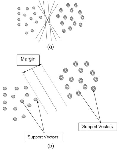
Fig. 1. (a) Hyper planes for linearly separable data, (b) Optimum hyper plane and support vectors [35].

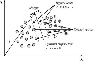
Fig. 2. Support vectors and optimum hyper plane for the binary case of linearly separable data sets [35].

Thus, determination of optimum hyper plane is required to solve optimisation problem given by:

min(0.5*||w||2 )                                               (4)

subject to constraints,

yi (w. xi + b ) ≥ -1   and yi  ε {+1, -1}                 (5)

As illustrated in Fig. 3 (a) [35], nonlinearly separable data is the case in various classification problems as in the classification of remotely sensed images using pixel samples. In such cases, data sets cannot be classified into two classes with a linear function in input space. Where it is not possible to have a hyper plane defined by linear equations on the training data, the technique can be extended to allow for nonlinear decision surfaces [38, 39].

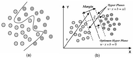
Fig. 3. (a) Separation of nonlinear data sets, (b) Generalisation of the solution by introducing slack variable for nonlinear data [35].

Thus, the optimisation problem is replaced by introducing  slack variable (Fig. 3(b)).

                                       (6)

subject to constraints,

                (7)

where C is a regularisation constant or penalty parameter. This parameter allows striking a balance between the two competing criteria of margin maximisation and error minimisation, whereas the slack variables  indicates the distance of the incorrectly classified points from the optimal hyper plane [40]. The larger the C value, the higher the penalty associated to misclassified samples [41].

When it is not possible to define the hyper plane by linear equations, the data can be mapped into a higher dimensional space (H) through some nonlinear mapping functions (Ф). An input data point x is represented as Ф(x) in the high-dimensional space. The expensive computation of (Ф(x).Ф(xi)) is reduced by using a kernel function [36]. Thus, the classification decision function becomes:

                  (8)

where for each of r training cases there is a vector (xi) that represents the spectral response of the case together with a definition of class membership (yi).αi (i = 1,….., r) are Lagrange multipliers and K(x, xi) is the kernel function. The magnitude of αi is determined by the parameter C [42]. The kernel function enables the data points to spread in such a way that a linear hyper plane can be fitted [43]. Kernel functions commonly used in SVMs can be generally aggregated into four groups; namely, linear, polynomial, radial basis function and sigmoid kernels. The performance of SVMs varies depending on the choice of the kernel function and its parameters.  A free and open source software – openModeller [44] was used for predicting the probable landslide areas. openModeller (http://openmodeller.sourceforge.net/) is a flexible, user friendly, cross-platform environment where the entire process of conducting a fundamental niche modeling experiment can be carried out. It includes facilities for reading landslide occurrence and environmental data, selection of environmental layers on which the model should be based, creating a fundamental niche model and projecting the model into an environmental scenario using a number of algorithms as shown in Fig. 4.

STUDY AREA AND DATA

The Uttara Kannada district lies 74°9' to 75°10' east longitude and 13°55' to 15°31' north latitude, extending over an area of 10, 291 km2 in the mid-western part of Karnataka state (Fig. 5). It accounts for 5.37 % of the total area of the state with a population above 1.2 million [45]. This region has gentle undulating hills, rising steeply from a narrow coastal strip bordering the Arabian sea to a plateau at an altitude of 500 m with occasional hills rising above 600–860 m. This district with 11 taluks, can be broadly categorised into three distinct regions –– coastal lands (Karwar, Ankola, Kumta, Honnavar and Bhatkal taluks), mostly forested Sahyadrian interior (Supa, Yellapur, Sirsi and Siddapur taluks) and the eastern margin where the table land begins (Haliyal, Yellapur and Mundgod taluks). Climatic conditions range from arid to humid due to physiographic conditions ranging from plains, mountains to coast.

Survey of India (SOI) toposheets of 1:50000 and 1:250000 scales were used to generate base layers – district and taluk boundaries, water bodies, drainage network, etc. Field data were collected with a handheld GPS. Environmental data such as precipitation of wettest month and precipitation in the wettest quarter were downloaded from WorldClim – Global Climate Data [http://www.worldclim.org/bioclim].

Precipitation (atmospheric water phenomena) is any product of the condensation of atmospheric water vapor that is pulled down by gravity and deposited on the Earth's surface such as rain.

Other environmental layers used in the model were obtained from USGS Earth Resources Observation and Science (EROS) Center based Hydro1Kdatabase [http://eros.usgs.gov/#/Find_Data/Products_and_Data_Available/gtopo30/hydro/asia] which are as follows:

 Aspect - describes the direction of maximum rate of change in the elevations or the slope direction. It is measured in positive integer degrees from 0 to 360, clockwise from north. Aspects of cells (pixels) of zero slope (flat areas) are assigned values of -1.

 DEM – is a digital representation of ground surface topography or terrain represented as a raster (a grid of squares) or as a triangular irregular network. DEMs are commonly built using remote sensing techniques or from land surveying.

 Flow accumulation (FA) - defines the number of pixels which flow into each downslope pixel. Since the pixel size of the HYDRO1k data set is 1 km, the flow accumulation value translates directly into upstream drainage areas in square kilometers. Values range from 0 at topographic highs to very large numbers (on the order of millions of square kilometers) at the mouths of large rivers.

 Flow direction (FD) - defines the direction of flow from each cell to its steepest down-slope neighbor derived from the hydrologically correct DEM. Values of flow direction vary from 1 to 255.

 Slope - describes the maximum change in the elevations between each pixel and its eight neighbors expressed in integer degrees of slope between 0 and 90.

Compound Topographic Index (CTI) - commonly referred to as the Wetness Index, is a function of the upstream contributing area and the slope of the landscape. It is calculated using the flow accumulation (FA) layer along with the slope as:

                                                     (9)

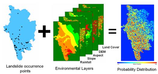
Fig. 4. Methodology used for landslide prediction in openModeller

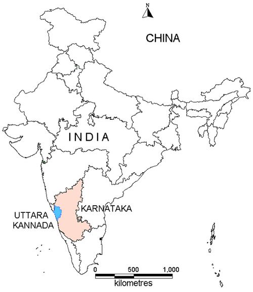
Fig. 5. Uttara Kannada district, Karnataka, India

In areas of no slope, a CTI value is obtained by substituting a slope of 0.001. This value is smaller than the smallest slope obtainable from a 1000 m data set with a 1 m vertical resolution.

The global land cover change maps were obtained from Global Land Cover Facility, Land Cover Change [http://glcf.umiacs.umd.edu/ services/landcoverchange/landcover.shtml; http://www.landcover.org/services/land coverchange/landcover.shtml].

The spatial resolution of all the data were 1 km. Google Earth data (http://earth.google.com) served in pre and post classification process and validation of the results. 125 landslide occurrence points of low, medium and high intensity were recorded using GPS from the field and published reports.

RESULTS AND DISCUSSION

Two different precipitation layers were used to predict landslides – precipitation of wettest month and precipitation in the wettest quarter of the year along with the seven other layers as mentioned in section III. Figure 6 (a) and (b) are the landslide probability maps using GARP and SVM on precipitation of wettest month. The landslide occurrence points were overlaid on the probability maps to validate the prediction as shown in Fig. 7. The GARP map had an accuracy of 92% and SVM map was 96% accurate with respect to the ground and Kappa values 0.8733 and 0.9083 respectively. The corresponding ROC curves are shown in Fig. 8 (a) and (b). Total area under curve (AUC) for Fig. 8 (a) is 0.87 and for Fig. 8 (b) is 0.93. Figure 6 (c) and (d) are the landslide probability maps using GARP and SVM on precipitation of wettest quarter with accuracy of 91% and 94% and Kappa values of 0.9014 and 0.9387 respectively.

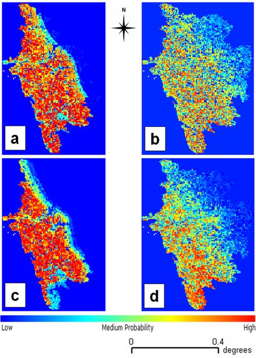
Fig. 6. Probability distribution of the landslide prone areas.

ROC curves in figure 8 (c) and (d) show AUC as 0.90 and 0.94. Various measures of accuracy were used as per [46] to assess the outputs. Table I presents the confusion matrix structure indicating true positives, false positives, false negatives and true negatives.

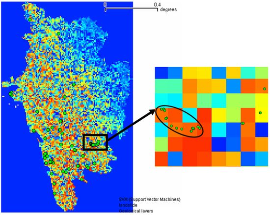
Fig. 7. Validation of the probability distribution of the landslide prone areas by overlaying landslide occurrence points

Confusion matrices were generated for each of the 4 outputs (Table II) and different measures of accuracy such as prevalence, global diagnostic power, correct classification rate, sensitivity, specificity, omission and commission error were computed as listed in Table III.

Fig. 8. ROC curves for landslide prone maps (a) GARP (b) SVM on precipitation of wettest month; (c) GARP and (d) SVM on precipitation of wettest quarter.

The results indicate that the output obtained from SVM using precipitation of the wettest month was best among the 4 scenarios. It maybe noted that the outputs from GARP for both the wettest precipitation month and quarter are close to the SVM in term of accuracy. One reason is that, most of the areas have been predicted as probable landslide prone zones (indicated in red in Fig. 6 (a) and (c)) and the terrain is highly undulating with steep slopes that are frequently exposed to landslides induced by rainfall. Obviously, the maximum number of landslide points occurring in the undulating terrain, collected from the ground will fall in those areas indicating that they are more susceptible to landslides compared to north-eastern part of the district which has relatively flat terrain.

Another case study of Kerala state, India was carried out with the same environmental layers along with 10 landslide occurrence points as shown in Fig. 9. The predicted output for precipitation in the wettest month is shown in Fig. 10 and precipitation in the wettest quarter is shown in Fig. 11 with an overall accuracy of 60%. The Kappa values for two cases were 0.966335 and 0.96532. The ROC curves are shown in Fig. 12 (a) and (b) with 0.97 AUC for both the cases respectively. The confusion matrix and statistics are presented in Table IV and V. The reason for low accuracy is the presence of only 10 occurrence points throughout the state. Also, the coarse resolution of the pixel may be attributed for poor accuracy. However, the Kappa value and the AUC are high which indicate that the probability distribution of the predicted points fall well within the occurrence points. It is another matter that the intensity of these landslide points may vary from low to medium to high. One potential limitation of the above data is their spatial resolution – 1 km. It is highly unlikely that landslides of this magnitude can occur in the study area. However, given the environmental layers along with the occurrence points, the probable areas of occurrence can be mapped with great certainty.

Table I : Confusion Matrix Structure

The movement of a slope is complex and it is induced or perturbed by many other factors besides rainfall such as groundwater data, soil moisture information, etc. which were not used in the prediction. It is known that there are accelerations of slope movements after intense rainfall, however, to what extent rainfall affects the slope movement remains unknown and the correlation between rainfall and the slope movement could be ambiguous in absence of detailed observations. Timely rainfall, soil moisture, grain-size, lithology, geological structure, seismological observations and the longer time intervals for which data are available can improve the accuracy of the model. Beyond their key role in identifying and mapping the landslides, the choice of the variables (environmental layers) used for the prediction are also closely involved. Some limitations of the data set cannot be overcome. In this study for example, no hydrological field data were available. However, significant results were obtained in the study because the variables most influential on landslide were used.

Natural disasters have drastically increased over the last decades. National, state and local government including NGOs are concerned with the loss of human life and damage to property caused by natural disasters. The trend of increasing incidences of landslides occurrence is expected to continue in the next decades due to urbanisation, continued anthropogenic activities, deforestation in the name of development and increased regional precipitation in landslide-prone areas due to changing climatic patterns [47]. The application of modern technologies required to control the effects of natural hazards including landslides must consider three significant factors - prediction, monitoring and conservation. In fact, the promotion of accessibility to urban facilities, such as homes and new roads in mountainous areas is difficult to achieve without considering geological and geotechnical factors to ensure that the development is pleasant and safe. Therefore, it is desired to have a notion about the main factors controlling the slope instability, assessing its severity, discriminating areas with presence/absence of landslides, updating and interpreting landslide data and determining areas that are prone to landslides. In this regard, the present work may be a contribution to the beginning of such disaster and mitigation studies.

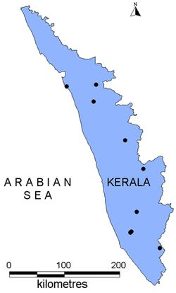
Fig. 9. Landslide occurrence points in Kerala

Table II: Confusion matrix for GARP and SVM Outputs for Uttara Kannada

Uttara Kannada		True Presence	TRUE ABSENCE	NUMBER OF USABLE PRESENCE	NUMBER OF USABLE ABSENCE
GARP with precipitation of wettest month	Predicted Presence	120	0	125	0
	Predicted Absence	5	0
SVM with precipitation of wettest month	Predicted Presence	118	0	125	0
	Predicted Presence	7	0
GARP with precipitation of wettest Quarter	Predicted Presence	118	0	125	0
	Predicted Presence	7	0
SVM with precipitation of wettest Quarter	Predicted Presence	117	0	125	0
	Predicted Presence	8	0

Table III : STATISTICS of GARP and SVM Outputs for Uttara kannada

Uttara Kannada	Prevalence (A+C)/N	Global diagnostic Power(B+D)/N	Correct Classification Rate(A+D)/N	Sensitivity A/(A+C)	Specificity D/(B+D)	Omission Error C/(A+C)	Commision Error B/(B+D)
GARP with precipitation of wettest month	-	-	0.96	0.96	-	0.04	-
SVM with precipitation of wettest month	-	-	0.94	0.94	-	0.06	-
GARP with precipitation of wettest Quarter	-	-	0.94	0.94	-	0.06	-
SVM with precipitation of wettest Quarter	-	-	0.94	0.94	-	0.06	-

* Key: A – True Positive, B – False Positive, C – False Negative, D – True Negative, N – Number of Samples.

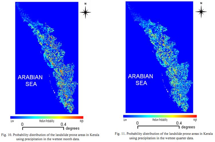
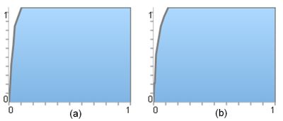
Fig. 12. ROC curves for the predicted landslide prone maps of Kerala. (a) using precipitation of the wettest month, (b) using precipitation of the wettest quarter.

Table IV : Confusion matrix for GARP Outputs for KERALA

Kerala		True Presence	TRUE ABSENCE	NUMBER OF USABLE PRESENCE	NUMBER OF USABLE ABSENCE
GARP with precipitation of wettest month	Predicted Presence	6	0	10	0
	Predicted Absence	4	0
GARP with precipitation of wettest Quarter	Predicted Presence	6	0	10	0
	Predicted Presence	4	0

Table V : STATISTICS of GARP Outputs for Kerala

Kerala	Prevalence (A+C)/N	Global diagnostic Power(B+D)/N	Correct Classification Rate(A+D)/N	Sensitivity A/(A+C)	Specificity D/(B+D)	Omission Error C/(A+C)	Commision Error B/(B+D)
GARP with precipitation of wettest month	-	-	0.6	0.6	-	0.4	-
GARP with precipitation of wettest Quarter	-	-	0.6	0.6	-	0.4	-

* Key: A – True Positive, B – False Positive, C – False Negative, D – True Negative, N – Number of Samples.

CONCLUSION

Landslides occur when masses of rock, earth or debris move down a slope.  Mudslides, debris flows or mudflows, are common type of fast-moving landslides that tend to flow in channels. These are caused by disturbances in the natural stability of a slope, which are triggered by high intensity rains. Mudslides usually begin on steep slopes and develop when water rapidly collects in the ground and results in a surge of water-soaked rock, earth and debris. Causes may be of two kinds: 1. Preparatory causes & 2: Triggering causes. Preparatory causes are factors which have made the slope potentially unstable. The triggering cause is the single event that finally initiated the landslide. Thus, causes combine to make a slope vulnerable to failure, and the trigger finally initiates the movement. Thus a landslide is a complex dynamic system. An individual ‘landslide’ characteristically involves many different processes operating together, often with differing intensity during successive years.

The primary criteria that influence landslides are precipitation intensity, slope, soil type, elevation, vegetation, and land cover type. The present study demonstrated the effectiveness of two pattern recognition techniques: Genetic Algorithm for Rule-set Prediction and Support Vector Machine. The landslide hazard prediction study conducted in Uttara Kannada and Kerala have shown that small datasets can yield landslide susceptibility maps of significant predictive power. The efficiency of the model has been demonstrated by the successful validation. However, when the predicted features may have different immediate causes, one should carefully avoid including triggering factors among the predictor variables since they restrict the scope of the prediction map and convey often a poorly constrained time dimension. Beyond the sample size, the reliability of the susceptibility map fundamentally depends on a good knowledge of which environmental variables act to determine landslides, and on the availability and the quality of the data. To be reliable or simply useful, the prediction map must also be appropriately validated. The
analysis showed that SVM applied on precipitation data of the wettest month with 96% accuracy was close to reality for Uttara Kannada district and GARP applied on precipitation data of the wettest quarter was more successful in identifying the landslide prone areas in Kerala.
VI. Acknowledgment

The environmental layers were obtained from WorldClim - Global Climate Data.  NRSA, Hyderabad provided the LISS IV data used for land cover analysis. We thank USGS Earth Resources Observation and Science (EROS) Center for providing the environmental layers and Global Land Cover Facility (GLCF) for facilitating the Land Cover Change product.

REFERENCES

1. S. Monia, G. Salvatore, N. Fernando, P. Andrea and R. C. Maria , “Pre-processing algorithms and landslide modelling on remotely sensed DEMs,” Geomorphology, vol. 113, pp. 110–125, 2009.
2. J. N. Hutchinson, “Morphological and geotechnical parameters of landslides in relation to geology and hydrology,” Proc. 5th Int. Symp. on Landslides, Lausanne, pp.  3–36, 1988.
3. R. H. Campbell, “Soil slips, debris flow, and rainstorms in the Santa Monica Mountain and vicinity Southern California,” US Geological Survey Professional Paper 851, 1975.
4. S. D. Ellen, G. K Wieczorek, “Landslides, floods and marine effects of the storm of January 3-5, 1982, in the San Francisco Bay Region, California,” United States Geological Survey Profession Paper, pp. 1434, 1988.
5. N. Caine, “The rainfall intensity–duration control of shallow landslides and debris flows,” Geografiska Annaler, vol. 62, pp. 23–27, 1980.
6. S. H. Cannon, and S. Ellen, “Rainfall conditions for abundant debris avalanches. San Francisco Bay Region, California,” California Geology,vol. 38, pp. 267–272, 1985.
7. G. F. Wieczorek, “Effect of rainfall intensity and duration on the debris flows in central Santa Cruz Mountains, California,” Geological Society of America Reviews in Engineering Geology,vol. 7, pp.93–104, 1987.
8. D. K. Keefer, R. C. Wilson, R. K. Mark, E. E. Brabb, W. M. Brown, S. D. Ellen, E. L. Harp, G. F. Wieczorek, C. S. Alger, R. S. Zatkin, “Real time landslide warning during heavy rainfall,” Science, col. 238, pp 921–925, 1987.
9. D. R. Montgomery, W. E. Dietrich, “A physically based model for the topographic control on shallow landsliding,” Water Resources Research, vol. 30 (4), pp. 1153–1171, 1994.
10. D. R. Montgomery, K. Sullivan, and H. M. Greenberg, “Regional test of a model for shallow landsliding,” Hydrological Processes, vol. 12, pp. 943–955, 1998.
11. R. M. Iverson, “Landslide triggering by rain infiltration,” Water Resources Research,vol. 36(7),1910.
12. Y. Hong, R. Adler, G. Huffman, “Evaluation of the potential of NASA multisatellite precipitation analysis in global landslide hazard assessment,” Geophysics Research Letter, vol. 33, L22402, 2006.
13. R. Rosso, M. C. Rulli, G. Vannucchi, “A physically based model for the hydrologic control on shallow landsliding,” Water Resources Research, 42, W06410, 2006.
14. G. B. Crosta, and P. Frattini, “Rainfall-induced Landslides and debris flows,” Hydrological Processes, 22,pp. 473-477, 2008.
15. W. Wu, R. Sidle, “A distributed slope stability model for steep forested basins,” Water Resources Research, vol. 31(8), pp. 2097–2110, 1995.
16. M. Casadei, W. E. Dietrich and N. L. Miller, “Testing a model for predicting the time and location of shallow landslide initiation in soil-mantled landscapes,” Earth Surface Processed and Landforms, 28, pp. 925–950, 2003.
17. T. L. Kwan, and H. Jui-Yi, “Prediction of landslide occurrence based on slope-instability analysis and hydrological model simulation,” Journal of Hydrology, vol. 375, pp. 489–497, 2009.
18. M. Borga, G. Dalla Fontana, D. Da Ros, and L. Marchi, “Shallow landslide hazard assessment using a physically based model and digital elevation data,” Environmental Geology,vol. 35, pp. 81–88, 1998.
19. A. Burton, and J. C. Bathurst, “Physically based modelling of shallow landslide sediment yield at a catchment scale,” Environmental Geology, vol. 35, pp. 89–99, 1998.
20. R. Romeo, “Seismically induced landslide displacements: a predictive model,” Engineering Geology, vol. 58, pp. 337–351, 2000.
21. K. J. Shou, and C. F. Wang, “Analysis of the Chiufengershan landslide triggered by the 1999 Chi-Chi earthquake in Taiwan,” Engineering Geology, vol. 68, pp. 237–250, 2003.
22. W. R. Lambe, R. V. Whitman, Soil Mechanics, 2nd ed. Wiley, New York, 1979.
23. R. D. Barling, I. D. Moore, and R. B. Grayson, “A quasi-dynamic wetness index for characterizing the spatial distribution of zones of surface saturation and soil water content,” Water Resources Research, vol. 30, pp. 1029–1044, 1994.
24. W. E. Dietrich, R. Reiss, M. Hsu, D. R. Montgomery, “A process-based model for colluvial soil depth and shallow landsliding using digital elevation data,” Hydrological Processes, vol. 9, pp. 383–400,1995.
25. M. Casadei, W. E. Dietrich, N. L. Miller, “Testing a model for predicting the timing and location of shallow landslide initiation in soil-mantled landscapes,” Earth Surface Processes and Landforms, vol. 28, pp. 925–950, 2003.
26. D. R. Montgomery, W. E. Dietrich, “A physically based model for the topographic control on shallow landsliding,” Water Resources Research, vol. 30, pp. 1153–1171, 1998.
27. J. DeGraff, H. Romesburg, “Regional landslide-susceptibility assessment for wildland management: a matrix approach” In: Coates, D., Vitek, J. (Eds.), George Allen and Unwin, “Thresholds in Geomorphology,” London, pp. 401–414, 1980.
28. A. Carrara, “Multivariate models for landslide hazard evaluation,” Mathematical Geology, vol. 15(3), pp. 403– 426,1983.
29. A. K. Pachauri, and M. Pant, “Landslide hazard mapping based on geological attributes,” Engineering Geology, vol. 32(1–2), pp. 81– 100, 1992.
30. P. M. Atkinson, and R. Massari, “Generalised linear modelling of susceptibility to landsliding in the central Appennines, Italy,” Computer and Geosciences,24(4), pp. 371–383, 1998.
31. K. Turner, and G. Jayaprakash, Introduction. In: Turner, A. K., Schuster, R.L. (Eds.), Landslides: Investigation and Mitigation,
32. Special Report, vol. 247. National Academic Press, Washington, DC, pp. 3– 12, 1992.
33. T. Ward, L. Ruh-Ming, and D. Simons, “Mapping landslide hazard in forest watershed,” Journal of Geotechnical Engineering Division,108(GT2), pp. 319– 324, 1988.
34. A. K. Pujari, Data Mining Techniques, University Press, Hyderabad, 2006.
35. D. R B. Stockwell, and D. P. Peters, “The GARB modeling system; Problems and solutions to automated spatial prediction,” International Journal of Geographic Information Systems, vol. 13, pp. 143-158, 1999.
36. T. Kavzoglu , I. Colkesen, “A kernel functions analysis for support vector machines for land cover classification”, International Journal of Applied Earth Observation and Geoinformation, vol 11, pp. 352-359, 2009
37. A. Mathur, and G. M. Foody, “Multiclass and binary SVM classification: Implications for training and classification users,” IEEE Geoscience and Remote Sensing Letters, vol. 5, pp. 241–245, 2008a.
38. A. Mathur, and G. M.  Foody, “A relative evaluation of multiclass image classification by support vector machines,” IEEE Transactions on Geoscience and Remote Sensing, vol. 42, pp.  1335–1343, 2004.
39. C. Cortes, and V.  Vapnik, “Support-vector network,” Machine Learning 20, pp 273–297, 1995.
40. M. Pal, P. M. Mather, “Support vector machines for classification in remote Sensing,” International Journal of Remote Sensing, vol. 26, pp. 1007–1011, 2003.
41. T. Oommen, D. Misra, N. K. C.  Twarakavi, A. Prakash, B. Sahoo, and S. Bandopadhyay, “An objective analysis of support vector machine based classification for remote sensing,”  Mathematical Geosciences, vol. 40, pp. 409–424, 2008.
42. F. Melgani, and L. Bruzzone, “Classification of hyperspectral remote sensing images with support vector machines,” IEEE Transactions on Geoscience and Remote Sensing, vol. 42, pp. 1778–1790, 2004.
43. A. Mathur, and G. M.  Foody, “Crop classification by support vector machine with intelligently selected training data for an operational application,” International Journal of Remote Sensing, vol. 29, pp. 2227–2240, 2008b.
44. B. Dixon, and N. Candade, “Multispectral land use classification using neural networks and support vectormachines: one or the other, or both?,” International Journal of Remote Sensing, vol. 29, pp. 1185–1206, 2008.
45. M. E. S Munoz, R. Giovanni, M. F Siqueira, T. Sutton, P. Brewer, R. S. Pereira, D. A. L. Canhos, and V. P Canhos, “openModeller- a generic approach to species’ potential distribution modeling,” Geoinformatica. DOI: 10.1007/s10707-009-0090-7.
46. T. V. Ramachandra and A. V. Nagarathna, “Energetics in paddy cultivation in Uttara Kannada district,” Energy Conservation and Management,vol. 42( 2), pp. 131-155, 2001.
47. A. H. Fielding, and J. F. Bell, “A review of methods for the assessment of prediction errors in conservation presence/absence models,” Environmental Conservation, vol. 24, pp. 38-49, 1997.
48. T V Ramachandra, M D Subashchandran and Anant Hegde Ashisar,. Landslides at Karwar, October 2009: Causes and Remedial Measures, ENVIS Technical Report: 32, Environmental Information System, Centre for Ecological Sciences, Bangalore, 2009.
49. A. K. Pachauri, and M. Pant, “Landslide hazard mapping based on geological attributes,” Engineering Geology, vol. 32(1–2), pp. 81– 100, 1992.
50. P. M. Atkinson, and R. Massari, “Generalised linear modelling of susceptibility to landsliding in the central Appennines, Italy,” Computer and Geosciences,24(4), pp. 371–383, 1998.
51. K. Turner, and G. Jayaprakash, Introduction. In: Turner, A. K., Schuster, R.L. (Eds.), Landslides: Investigation and Mitigation,
52. Special Report, vol. 247. National Academic Press, Washington, DC, pp. 3– 12, 1992.
53. T. Ward, L. Ruh-Ming, and D. Simons, “Mapping landslide hazard in forest watershed,” Journal of Geotechnical Engineering Division,108(GT2), pp. 319– 324, 1988.
54. A. K. Pujari, Data Mining Techniques, University Press, Hyderabad, 2006.
55. D. R B. Stockwell, and D. P. Peters, “The GARB modeling system; Problems and solutions to automated spatial prediction,” International Journal of Geographic Information Systems, vol. 13, pp. 143-158, 1999.
56. T. Kavzoglu , I. Colkesen, “A kernel functions analysis for support vector machines for land cover classification”, International Journal of Applied Earth Observation and Geoinformation, vol 11, pp. 352-359, 2009
57. A. Mathur, and G. M. Foody, “Multiclass and binary SVM classification: Implications for training and classification users,” IEEE Geoscience and Remote Sensing Letters, vol. 5, pp. 241–245, 2008a.
58. A. Mathur, and G. M.  Foody, “A relative evaluation of multiclass image classification by support vector machines,” IEEE Transactions on Geoscience and Remote Sensing, vol. 42, pp.  1335–1343, 2004.
59. C. Cortes, and V.  Vapnik, “Support-vector network,” Machine Learning 20, pp 273–297, 1995.
60. M. Pal, P. M. Mather, “Support vector machines for classification in remote Sensing,” International Journal of Remote Sensing, vol. 26, pp. 1007–1011, 2003.
61. T. Oommen, D. Misra, N. K. C.  Twarakavi, A. Prakash, B. Sahoo, and S. Bandopadhyay, “An objective analysis of support vector machine based classification for remote sensing,”  Mathematical Geosciences, vol. 40, pp. 409–424, 2008.
62. F. Melgani, and L. Bruzzone, “Classification of hyperspectral remote sensing images with support vector machines,” IEEE Transactions on Geoscience and Remote Sensing, vol. 42, pp. 1778–1790, 2004.
63. A. Mathur, and G. M.  Foody, “Crop classification by support vector machine with intelligently selected training data for an operational application,” International Journal of Remote Sensing, vol. 29, pp. 2227–2240, 2008b.
64. B. Dixon, and N. Candade, “Multispectral land use classification using neural networks and support vectormachines: one or the other, or both?,” International Journal of Remote Sensing, vol. 29, pp. 1185–1206, 2008.
65. M. E. S Munoz, R. Giovanni, M. F Siqueira, T. Sutton, P. Brewer, R. S. Pereira, D. A. L. Canhos, and V. P Canhos, “openModeller- a generic approach to species’ potential distribution modeling,” Geoinformatica. DOI: 10.1007/s10707-009-0090-7.
66. T. V. Ramachandra and A. V. Nagarathna, “Energetics in paddy cultivation in Uttara Kannada district,” Energy Conservation and Management,vol. 42( 2), pp. 131-155, 2001.
67. A. H. Fielding, and J. F. Bell, “A review of methods for the assessment of prediction errors in conservation presence/absence models,” Environmental Conservation, vol. 24, pp. 38-49, 1997.
68. T V Ramachandra, M D Subashchandran and Anant Hegde Ashisar,. Landslides at Karwar, October 2009: Causes and Remedial Measures, ENVIS Technical Report: 32, Environmental Information System, Centre for Ecological Sciences, Bangalore, 2009.