| Sahyadri Conservation Series - 7 |
ENVIS Technical Report: 28, February 2012 |
 |
Landslide Susceptible Zone Mapping in Uttara Kannada, Central Western Ghats |
 |
Energy and Wetlands Research Group, Centre for Ecological Sciences,
Indian Institute of Science, Bangalore – 560012, India.
*Corresponding author: cestvr@ces.iisc.ac.in
CASE STUDY: SHARAVATHI RIVER BASIN
OBJECTIVE
The aim of the study is to map landslide prone zones in the Sharavathi river basin (Uttara Kannada and Shimoga districts, Karnataka State) using the remote sensing data and GIS techniques. Specific objectives are:
- Identification of causal factors of landslides using information collected from fieldwork, government agencies and remote sensing.
- Spatial mapping of landslide prone zones, and
- Assessment of the extent of damage due to landslide hazards.
Remote sensing data with better spectral and spatial resolutions along with data of soil, land use, climate, etc. and GIS would help in preparing the landslide distribution map. This involves:
- Generating a spatial database identifying the base layers that play a role in landslide susceptibility pertaining to the study area.
- Creating a landslide database to identify the causative factors of landslide slumps and creeps in the study area, through mapping, gathering information in the field and remote sensing approaches.
- Evaluating the direct relationship between the causative factors of hill slope instability and the combination of landslide susceptibility from contributing base layers.
- Creation of a landslide hazard map using statistical data generated to create landslide susceptible polygons.
- Evaluating human hazards and suggesting corrective measures to minimise future risks towards areas of human habitation, infrastructure and transportation.
METHOD
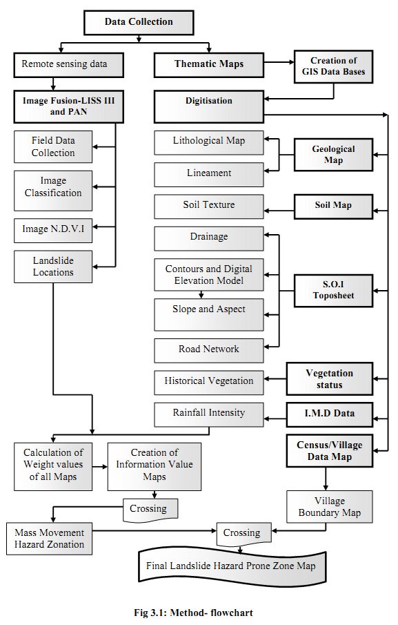
The aim of this study is to identify the causal factors of landslides, using information collected from fieldwork, GIS and remote sensing sources and to identify slide prone zones and assess human hazard in the Sharavathi River Basin. Methods as outlined in Figure 3.1 involved to achieve the objectives are:
- Pre Fieldwork: Review of literature; Collection of secondary data; Collection of topo-sheets on 1:50,000 scales.
- Field investigation: Identification of landslides in the study area and collection of their coordinates using GPS; Collection of attribute data; Collection of training data (GCP’s) for supervised classification of remote sensing data; Documentation of sensitive areas with the feedback from local people; Identification of environmentally unsound anthropogenic activities such as diversion of streams, road cuts, etc.
- Post Fieldwork: Creation of Digital database of secondary data and toposheets, etc.; Geo-referencing of maps and images; Digitisation of cadastral maps; supervised classification of remote sensing data; generating Digital elevation model (DEM), slope and aspect maps of study area; Preparation of final map tables and diagrams.
Data Used
- IRS 1C/1D LISS III MSS data (temporal data) IRS 1C/1D PAN data
to see the spatial and temporal changes.
- Survey of India Toposheets on 1:50000 scales to create GIS base layers.
- Geological map with attribute data from Karnataka State Remote Sensing Applications Centre (KSRSAC).
- Soil map along with attribute data from National Bureau of Soil survey and Landuse Planning.
- Meteorological data from India Meteorological Department, Pune.
- Rainfall data of Sub-basins from Karnataka Power Corporation Limited (KPCL), Agriculture Departments (Honnavar, Kumta, Siddapur, Sagar and Hosanagara).
- Literature that provide an understanding of the concept and advancement in this area of research.
Software Used
IDRISI 3 for D.E.M, fusion of PAN & LISS-III, images raster analysis and image analysis and Arc View 3.2, MAPINFO 6.0 for vector analysis.
STUDY AREA
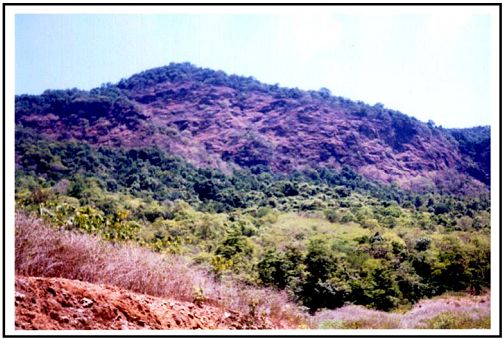
This study was carried out in the Sharavathi river basin, one of the west flowing rivers of Karnataka (figure 4.2). This river has been utilised for power generation through two reservoirs (at Linganamakki and at Gerusoppa). It is located at Shimoga and Uttara Kannada Districts of Karnataka State. Shimoga district is situated roughly in the mid-south-western part of the state. Sharavathi River Basin, is situated in the north part of the Western Ghats, a continuous range of hills that act as a drainage divide, separating the South Deccan Plateau from the Coastal Plain. The district is situated between 13o27’ and 14o39’ north latitude and 74o38’ and 76o04’ east longitude, bestowed with abundant natural resources. The general elevation along the Sharavathi River Basin is about 640 metres above sea level in the west, falling to about 529 meters in the east. The important rivers that flow in the district are Tunga, Bhadra, Sharavathi, Kumudwathi and Vardha. The Sharavathi River discharges into the sea at Honnavar in North Kannara. The Karnataka Power Corporation Limited (KPCL) has constructed a dam across the river near Linganamakki, one of the oldest hydroelectric power projects in India. The entire study area falls in mid region of Western Ghats having steep and undulating terrain. The area under study is the Sharavathi river basin with catchment area of 2924 km2. Figure 4.1 illustrates that Sharavathi basin as a hydrological unit comprising of geographical, ecological and cultural diversities.

STUDY AREA: Sharavathi River Basin, Karnataka
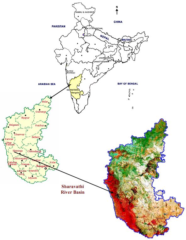
Fig 4.2: Sharavathi river basin, Karnataka, India
- Accessibility: This study area is well connected by road and rail to several major cities of Karnataka and neighbouring states and an important railhead of the newly constructed Konkan railway connects this coastline; the newly built bridge across the Sharavathi river, dominates the landscape. The study area is about 350 km from Bangalore, 200 km from Goa and is less than 60 km from Shimoga. Except some hilly areas, almost the entire area is well connected by the metalled roads and water ferry. Some villages inside the forest area are well connected with ordinary roads. The Bangalore-Goa highway passes through the study area. Rest of the hilly areas are well connected with non-metalled or metalled roads. Many foot tracks and water ferries are also present in the hilly terrain.
- Physiography: Physiographically, the study area encompasses low-lying flat terrain to highly undulating hilly ranges. The lowest elevation observed in the study area is around 20 m above sea level that is near the Arabian Sea and the highest relief is around 1340 m in the southern part of upstream area and northern part of downstream area. The study area is part of the rugged terrain of Western Ghats of southwest Shimoga and southeast Uttar Kannada. This region, by virtue of its geographical location in the central Western Ghats, and heterogeneity in the terrain and micro-climatic variations support a rich diversity of flora and fauna.
The Karnataka Power Corporation Limited has constructed a dam across the river in 1964 near Linganamakki, which is at present one of the oldest hydroelectric power projects in India. The dam is located at about 14°41'24'' N latitude and 74° 50’54’’ E longitudes with an altitude of 512 m. The water from Linganamakki dam flows to Talakalale Balancing Reservoir through a trapezoidal canal with a discharge capacity of 175.56 cu m. The length of this channel is about 4318.40 m with a submersion of 7.77 sq. km. It has a catchment area of about 46.60 sq.km. The gross capacity of the reservoir is 129.60 cu m. Sharavathi River alone, in its fullest potential, accounts for an estimated electricity generation of about 6,000 million units (kWh) per annum. Due to the hilly terrain, the submergence and consequent increase in water-spread area due to the dam and Sharavathi River has resulted in the creation of several islands distributed throughout the reservoir. There are about around 125 islands with sizes ranging from 2-3 sq. km to less than 25 sq. km. In most of the submerged areas the highlands and hilltops protrude out of the water-filled surroundings as islands.
- Climate and Rainfall: The area has well-marked seasons of monsoon from May-June to October, winter from November to January and summer from February to May. The temperature ranges from 10°C in winter nights to 32°C in summer. The weather is humid throughout the year with a variation of average rainfall from 1200 mm to 2600 mm in different parts of the catchment. Relative humidity is generally high at around 75% during southwest monsoon season and moderate during the rest of the year. Humidity during summer afternoons is relatively low. Average minimum and maximum temperature are about 15ºC and 38ºC respectively. Wind is generally moderate with some increase in strength during monsoon months and is mainly South-westerly in the mornings and between Northeast and Southeast in the afternoons. There is rapid increase of temperatures after January. April is usually the hottest month with the mean daily maximum temperature at 35.8°C and the mean daily minimum temperature at 22.2°C. In December, the mean daily maximum temperature is 29.2°C and the mean daily minimum temperature is 14.9°C.
The climate of the area is dominated by the southwest monsoons during June to August that bring "incessant rainfall" depositing 5000 to 8000 mm per annum in the Sharavathi catchment basin. The annual normal rainfall in the area is 1526 mm and some station locations even experience an annual rainfall of 2875 mm. Southwest monsoon starts normally from the second week of June and peaks during July and August. During monsoon, the water level reaches its peak leaving the top of the hills and hillocks on which the vegetation thrives. However, summer season interconnects the Islands as the water level recedes. As a result of this heavy rainfall the Western Coast drainage basin is home to one of the major tropical evergreen forest regions in India, which provide much of the timber to the economies of Sagar and Hosanagara taluks.
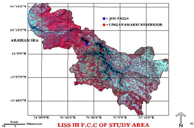
- Drainage: The Sharavathi river originating in the central Western Ghats runs through the districts of Shimoga and Uttara Kannada. The river has a catchment area of about 3600 sq. km. Sharavathi River Basin lies entirely in the Western Coast drainage basin bordered by the eastern drainage divide to the east and the west escarpment to the west, which is most visibly pronounced at Jog Falls where the river drops precipitously from a height of 255 m into a deep gorge and it is characterised by very steep "V" shaped sub parallel ravines formed by steep, fast, west flowing streams. It is one of the most spectacular scenic places of the Western Ghats. The river water is stored in three major reservoirs, namely, at Linganamakki (14º10’24” N, 74º50’54” E), Talakalale (14º11’10” N, 74º46’55” E) and Gerusoppa (14º15’N, 74º39’ E). The areas submerged for these reservoirs are 326.34, 7.77 and 5.96 km2 respectively. The river, and its tributaries and numerous streams run through the rugged terrain of the Ghats. The river, which takes birth at Ambuthirtha in Thirthahalli taluk, flows northwesterly for 130 km to join the Arabian Sea at Honnavar, in Uttara Kannada district. The major tributaries of the river are, Nandiholé, Haridravathi, Sharmanavathi, Hilkunjiholé, Nagodiholé, Hurliholé, Yenneholé, Mavinaholé, Gundabalaholé, Kalkatteholé, and Kandodiholé.
- Soil Texture: Soils in the region are mainly lateritic in origin and tend to be predominantly acidic and reddish in colour. In Sagar taluk, soils are 94% acidic while in Hosanagara taluk the percentage drops slightly to 76%. Nitrogen and phosphorous concentrations range from moderate to very low for Sagar and Hosanagara taluks respectively, while in both the taluks, soils are deficient in phosphorous (Karnataka State Gazetteer, 1975). Soils are rich in organic matter and low in phosphate, nitrate and sulphate concentration, while pH ranges from 5.5 - 6.8. The sediments have low sulphate (0.191 - 0.68 mg/gm), nitrate (0.0 - 0.0007 mg/gm) and phosphate (0.00024 - 0.001 mg/gm) concentrations, indicating close correlation between sediment and catchment soil. The sediment samples are rich in organic carbon and the elements like Na, K, Ca, and Mg are found well within the prescribed standards. Bulk density of sediments in streams of the western region indicates their porous condition (0.783 - 0.983 gm/cm3) while in the eastern side they are less porous (1.23 - 1.475 gm/cm3).
- Geological Parameters: The Karnataka Carton, similar to other shield areas in the world, consisting of geologically stable rocks of Achaean age mainly dominates the geology of the region. Geological units include the Dharwar Schist Belt and the Older Gneiss Complex. Due to the humid climate of the region substantial intense in-situweathering has taken place, leading to extensive creation of laterite over much of the terrain, making it the third major geological unit in the study area. The ghat area extending for a longer length lies parallel to the west coast, forming one of the most magnificent escarpments of tertiary age. Sediments of Palaeocene and younger ages are deposited in the graben area (Figure 4.3), developed at the west of the present day west coast of India. As the area is having a prominence of hilly terrain, it encompasses lots of lineament cracks, which play a vital role in the creation of loose slopes for the failure.
Fig 4.3: Western Ghats - study area, the faulted margin of the west coast and Arabian sea filling up the graben
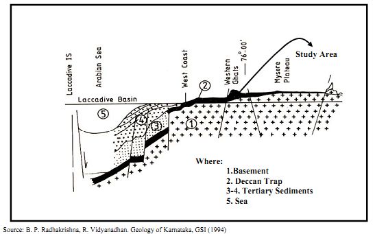
Figure 4.4 below shows a topographical undulation in the terrain with higher mountainous area along with geological unconformities of folds and faults.
- Vegetation - Flora and Fauna
Sharavathi river upper and lower catchment areas have a variety of natural vegetation ranging from the climax tropical evergreen to semi-evergreen forests with around 16% of them along the high rainfall areas of the main hill ranges of the Western Ghats to the moist deciduous forests, and around 25% of them in the undulating plains and low hills along the eastern drier tracts of the river basin. The landscape everywhere is in fact a mosaic of a variety of elements caused by human impacts through historical times to the current period. Around 21% of all vegetation consists of grassland, scrub, and cultivable waste. River Basin is also rich in animal diversity as it covers a large part of Sharavathi Wildlife Sanctuary. The region is also adjacent to Mookambika Wildlife Sanctuary of Udupi District and Shettihalli Wildlife Sanctuary of Shimoga District. Due to rising human pressures including creation of numerous monoculture plantations, many of the migratory paths of the animals are disrupted.
REMOTE SENSING, DIGITAL IMAGE PROCESSING AND GIS
Remote Sensing data:
The data used for the study area to analyse the Landslide Prone Zone Mapping using Remote Sensing and GIS Technique is mainly IRS-1C: LISS-III and PAN images were acquired from NRSA (National Remote Sensing Agency). Table 5.1 lists the spectral and spatial resolutions along with other details.
Table 5.1: Technical specification of LISS III and PAN imagery
| IRS 1-C |
| Specifications |
LISS-III |
PAN |
| Spatial resolution (m) |
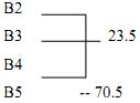 |
5.8 |
| Spectral bands |
B2- 0.52 to 0.59
B3- 0.62 to 0.68
B4- 0.77 to 0.86
B5- 1.55 to 1.70 |
0.5 - 0.75 |
| Swath (km) |
140 |
70 |
| Repetivity |
24 days |
24 days |
| Revisit |
5 days |
5 days |
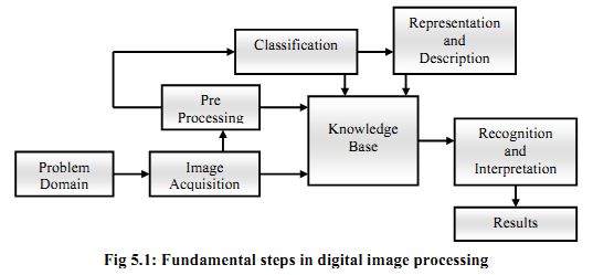
Digital Image Processing: Digital image processing encompasses four major areas of spatial data analysis (Figure 5.1), which are:
- Image Restoration or Pre-processing- Computer routines correct a degraded digital Image to its intended form, which is usually a precursor to the following steps.
- Image Enhancement- Computer routines improve the detestability of objects or patterns in a digital image for visual interpretation.
- Image Classification- Quantitatively classifying or identifying objects or patterns on the basis of their multi spectral radiance values.
- Data-Set Merging- Computer routines integrate multiple sets of data from the same location such that appropriate measurements can be made.
Geographical Information System (GIS)
These information systems aid to create, manipulate, store and use spatial data much faster compared to conventional methods. The factors, which are included in determining the occurrence of landslide hazard, are topography (slope angle and aspect), geology, geological-structures, soil texture and rainfall intensity. Along with these, other factors that can determine the degree of disaster include nature conditions, land-use, and anthropogenic activities i.e. the distribution of buildings and roads. GIS along with terrain analysis can be used for setting up a database.
TERRAIN ANALYSIS AND GIS DATA GENERATIONS
1. Terrain Analysis: The topographic data required a more extensive treatment. From the Survey of India toposheet (1:50000 scale) the contours are digitised at 20-metre intervals. Digital elevation model (DEM) “which is a digital cartographic representation of the elevation of the terrain at regularly spaced intervals in X and Y directions using Z values referenced to a common vertical datum i.e. Height” was developed to get the 3-D visualisation of the whole terrain. The DEM can be generally as Triangular Irregular Network (TIN), which is based on an irregular array of points, forming a sheet of non-overlapping contiguous triangle facets or Gridded Surfaces (DEMs, DTMs) as a rectangular array of cells storing the elevation value for the centroid of the cell. The study area is having diverse topographic features from sea level (0 m) to 1340 m height in extreme hilly terrain areas and Gridded surface DEM is used for model generation. Slope is a calculation of the maximum rate of change across the surface either from cell to cell in a gridded surface or of a triangle in a TIN. Aspect identifies the steepest downslope across the surface, always considered to be a significant determinant of landslide hazard. Higher the slope, there is a greater chance of occurrence of landslide. The digital elevation model developed using the topographic data is used to derive a corresponding slope and aspect model. These groups are generalisations about slopes in the study area, creating classes that are termed flatter due to lower slope value and steeper resulting from higher slope value in the slope zone legend. Slope is either calculated as percent of slope or degree of slope. An aspect map is also derived from elevation values in DEM. The aspect value assigned to each cell in an aspect map helps in identifying the direction (north, south, etc.) to which the side cell is oriented and landslide occurred. The topographic data contours are shown in the Figure 6.1 below, which helped in DEM, 3-D perspective (as shown in Figure 6.1 a and 6.1 b in the annexure), slope and Aspect Map creation.
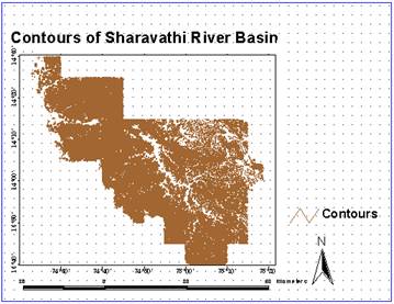
Fig 6.1: Contours of Sharavathi river basin
Existing Landslide: Field visit to existing landslide points helped in collection of GPS readings for areas under landslide, determination of soil bulk density of the landslide site, area affected due to the landslide and sample for soil texture and lithology. These details are used in determination of various aspects, which can be used in calculating the weights that helps in preparing the map of susceptible landslide areas. The existing landslide map is prepared on the basis of observations collected in the field to know the exact location of landslide. This is overlaid on the geo-referenced remote sensing data, which helped in identifying the parameters responsible on the basis of tone and texture in the image. With this information, probable area of landslide can be mapped. The existing landslide map of the study area is shown below in Figure 6.2. The location details (geo co-ordinates) of the landslide locations are given in Table 6.1.
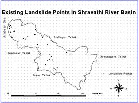
Fig 6.2: Existing landslide points in Sharavathi river basin
Base Layers - Road Network
Mass wasting and landslides can also occur in response to modification of hill slope conditions and hydrology. Road density, road network and road location can set the stage for mass wasting to occur especially when the site has an inherent propensity for sliding. Often there is a combination of causes for failures that involve increased water in the slide mass itself, which adds weight and reduces the soil strength by increased pore pressure. This in combination with the loss of support due to a road cut at the toe of a slide can result in mass wasting. In some cases, simply the loss of support at a road cut can cause a slide where increased water may not be a factor. Roads have been built across the toe of slides, which have removed this support giving or an otherwise stable hill slope into a chronic source of sediment and a site for mass wasting (Figure 6.3). Experimental studies showed that landslides, especially from poorly designed roads during major storms, pulsed large amounts of sediment in brief episodes, while surface erosion from roads and clear cuts was more chronic.
Table 6.1: Landslide location details
| Sr. No |
NORTHING |
EASTING |
Length*Width*Height (m) |
| 1 |
14° 12' 31.76 |
74° 51' 4.14 |
250* 50* 50 |
| 2 |
14° 8' 36.70 |
74° 43' 19.67 |
200* 200*100 |
| 3 |
14° 14' 33.54 |
74° 27' 13.94 |
200*50*100 |
| 4 |
14° 13' 30.18 |
74° 35' 42.58 |
50*100*100 |
| 5 |
14° 13' 42.78 |
74° 34' 16.68 |
100*100*100 |
| 6 |
14° 14' 51.03 |
74° 37' 1.09 |
200*25*25 |
| 7 |
14° 3' 1.08 |
74° 51' 13.6 |
200*100*100 |
| 8 |
14° 3' 57.20 |
74° 49' 54.08 |
100*50*50 |
| 9 |
14° 0' 37.51 |
74° 48' 58.78 |
200*50*75 |
| 10 |
13° 55' 43.53 |
74° 52' 48.82 |
150*50*50 |
| 11 |
13° 55' 8.94 |
74° 53' 56.4 |
50*50*100 |
| 12 |
13° 56' 1.79 |
74°54' 46.8 |
150*50*100 |
| 13 |
13° 57' 55.15 |
74° 47' 42.21 |
100*50*100 |
| 14 |
14° 1' 11.74 |
74° 50' 5.78 |
100*25*50 |
| 15 |
14° 0' 46.98 |
74° 51' 59.43 |
250*100*150 |
| 16 |
14° 0' 48.31 |
74° 52' 7.96 |
150*75*100 |
| 17 |
14° 10' 17.25 |
74° 48' 59.04 |
50*50*100 |
| 18 |
14° 4' 52.96 |
74° 44' 32.60 |
50*50*50 |
| 19 |
14° 4' 52.53 |
74 44' 37.10 |
200*50*100 |
| 20 |
14° 4' 22 |
75° 3' 3.85 |
100*100*50 |
| 21 |
14° 5' 20.5 |
75° 0' 34.2 |
500*100*100 |
| 22 |
14° 15' 30 |
74° 45' 55 |
50*25*100 |
| 23 |
14° 16' 15.88 |
74° 41' 28.45 |
100*25*25 |
| 24 |
14° 16' 11 |
74° 41' 3 |
150*25*50 |
| 25 |
14° 18' 20 |
74° 29' 10 |
250*25*50 |
| 26 |
14° 18' 14 |
74° 29' 3 |
250*25*50 |
| 27 |
14° 14' 46.24 |
74° 27' 22 |
250*50*50 |
| 28 |
14° 14' 36.63 |
74° 27' 41.50 |
300*100*200 |
| 29 |
14° 17' 38.68 |
74° 26' 33.75 |
500*500*100 |
| 30 |
14° 17' 36.85 |
74° 26' 42.82 |
500*500*100 |
| 31 |
14° 18' 1.62 |
74° 28' 34 |
200*50*100 |
| 32 |
14° 21' 14.32 |
74° 25' 55.3 |
300*50*100 |
| 33 |
14°21' 43.2 |
74°26' 34.51 |
300*50*100 |
| 34 |
14°21' 57.45 |
74°26' 13.38 |
200*50*100 |
| 35 |
14°20' 48.08 |
74°27' 14.25 |
200*50*50 |
| 36 |
14°19' 53.04 |
74°25' 58.58 |
200*100*200 |
| 37 |
14° 10' 7.5 |
74° 42' 55.26 |
500*100*50 |
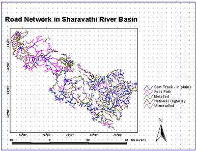
Fig 6.3: Road network in Sharavathi river basin
Village Boundary, Settlement Location and Population
The village boundary, settlements and population map in the study area are also prepared using the village taluk maps, toposheets and census data (1991). This helps in identifying the socio-economic status of the region and the extent of damage in case of hazards (people affected, etc.). This also would aid in quantifying the extent of damage due to natural disaster and remedial measures to be undertaken. The village boundary map and settlement location map of the study area are shown below in Figures 6.4 and 6.5.
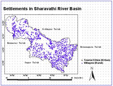
Fig 6.4: Settlements in Sharavathi river basin
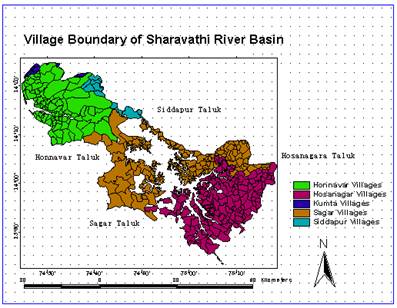
Fig 6.5: Village boundary of Sharavathi river basin
Soil Characteristics
Soil is the product of the weathering of rock and sediments. It is also referred as “relatively loose agglomerate of mineral and organic materials and sediments found above bedrock” (Holtz and Kovacs, 1981). The soils of the district are basically derivatives of Dharwar system - ancient metamorphic rocks in India; rich in iron and Mg. Exposed lateritic rocks along the coastal hills are very infertile and almost barren. During the last 15 years, most of these hills have been brought under forest plantation dominated by Acacia auriculiformis. The various types of soil existing in the study area are as shown in the soil characteristic map in Figure 6.6. Soils are divided on the basis of certain properties as these play a vital role in deciding the susceptibility of a probable landslide. They are classified into three sizes—sand, silt and clay and possess certain specific properties, namely,
- Sandy texture soils: The sandy group includes the sand and loamy sand soil textural classes. The soil is loose when dry and sand particles are plainly visible. It is not at all sticky when wet, but feels very gritty. It cannot be moulded or rolled into sausages. High proportions of fine sand can be identified by comparative lack of grittiness.
- Coarse loamy texture soils: The coarse loamy group includes sandy loam and loam soil textural classes. The sand fraction is plainly visible when dry, but the soil is not so loose. When moist the soil feels very gritty between the fingers. It can just be moulded, but does not retain any impressed shape easily. It does not stick to the fingers very much and cannot be rolled into sausages..
- Fine loamy texture soils: The fine loamy group includes silt, silt loam, sandy clay loam, clay loam, and silty clay loam textural classes. The sand fraction is more difficult to distinguish when dry. The soil is slightly gritty when moist. It moulds readily and retains impressed shapes. It sticks to the fingers slightly. It will roll into sausages with difficulty but the sausages will break up if an attempt is made to roll them to diameters less than 2 mm. Clay loam soil is rather hard when dry. It is distinctly sticky when wet. Only pressing the moist soil hard between the fingers can identify the sand fraction. It will roll into sausages with ease and the sausages will not break up so easily as loam as the diameter falls below 2 mm.
- Clayey texture soils: The clayey group includes sandy clay, silty clay, and clay textural classes and shall be considered provisionally suitable with respect to texture. Clay soil is very hard when dry and very sticky when moist. It is very difficult to detect the sand fraction by pressing the moist soil between the fingers. The soil can be rolled easily into fine sausages of less than 2 mm diameter. The soil particles vary in shape from spherical to angular. They differ in size from gravel and sand to fine clay. Various types of soil and their composition can be seen tabulated in Table 6.2 below.
(http://www.dot.ca.gov/hq/oppd/hdm/pdf/chp0840.pdf).
Table 6.2: Soil composition
| Soil Class |
Percent sand |
Percent silt |
Percent clay |
| Clean Sand |
80-100 |
0-20 |
0-20 |
| Sandy Loam |
50-80 |
0-50 |
0-20 |
| Loam |
30-50 |
30-50 |
0-20 |
| Clay Loam |
20-50 |
20-50 |
20-30 |
| Sandy Clay |
50-70 |
0-20 |
30-50 |
| Silty Clay |
0-20 |
50-70 |
30-50 |
| Clay |
0-50 |
0-50 |
30-100 |
Along with these physical compositions, soils also have diverse characteristics in their percentage inorganic composition, which also determines the stability and durability of the soil. The inorganic composition is shown in Table 6.3:
Table 6.3: Percentage inorganic composition of representative soil
| Type |
SiO2 |
Al2O3 |
Fe2O3 |
MnO |
CaO |
MgO |
K2O |
Na2O |
P2O5 |
| Sandy |
91.72 |
2.92 |
2.36 |
- |
0.35 |
0.78 |
0.33 |
0.08 |
0.08 |
| Sandy loam |
84.84 |
5.30 |
4.52-10.89 |
- |
0.06-0.91 |
0.29-0.52 |
0.16-0.71 |
0.03 |
0.10-0.34 |
| Loam |
86.98 |
4.10 |
3.52-10.89 |
- |
0.06-0.42 |
0.29-1.29 |
0.56-0.71 |
- |
0.06-0.34 |
| Silt loam |
86.49 |
9.16 |
7.00 |
0.21 |
0.14 |
0.90 |
1.85 |
- |
0.24 |
| Clay |
65.16 |
13.76 |
9.27 |
0.25 |
1.09-2.18 |
1.60-2.47 |
0.14-1.60 |
0.01 |
0.23 |
Soil texture is a measure of how much sand, silt, and clay a particular type of soil contains. Soil texture is important because it determines the porosity and permeability (i.e. how fast water drains through a soil and how much water a soil can hold). Slope and aspect affect the moisture and temperature of soil. Steep slopes facing the sun are warmer. Steep soils get eroded and lose their topsoil as they form. Sand is the largest size particle in soil that is 0.05-2 mm in diameter. Clay is less than 0.002 mm in diameter. Clay particles are extremely small, and can be seen only through an electron microscope.
Clay mineralogy along with soil texture is also important as the mineralogy of the clay-sized fraction determines the degree to which some soils swell when wet and thereby affect the size and number of pores available for movement of sewage effluent through the soil. There are two major types of clays, including the 1:1 clays, such as Kaolinite, which do not shrink or swell extensively when dried or made wet; and the 2:1 clays, including mixed mineralogy clays, such as clays containing both Kaolinite and Montmorillonite that shrink and swell when dried and made wet. The type of clay minerals in the clay-sized fraction are determined by a field evaluation of moist soil consistence or of wet soil consistence using Soil Taxonomy. The soils are examined for certain parameters, which are shown in Table 6.4.
Table 6.4: Parameters of landslide soil analysis
| Sr. no |
Landslide Name |
Soil Colour |
pH |
Bulk density
g/cc |
WHC % |
K2O kg/ha |
Moisture% |
| 1 |
Kauti |
Red |
5.3 |
1.96 |
35.27 |
46.4 |
25.74 |
| 2 |
Yellagadde |
Brown sandy |
4.8 |
2.02 |
14.54 |
45.1 |
13.86 |
| 3 |
Athavadi |
Brown sandy |
5.4 |
1.89 |
14.43 |
199.6 |
10.50 |
| 4 |
Belmakki |
Red |
5.5 |
1.89 |
29.47 |
14.2 |
28.98 |
| 5 |
Kapegi |
Red |
5.4 |
2.09 |
19.64 |
21.9 |
16.57 |
| 6 |
Suralli |
Brown |
5.6 |
1.99 |
34.00 |
12.9 |
19.36 |
| 7 |
Samse |
Brown |
6.0 |
2.12 |
31.37 |
15.5 |
24.61 |
| 8 |
Kalgalli |
Red |
5.5 |
1.93 |
23.86 |
106.9 |
22.49 |
| 9 |
Near Nittur |
Brown |
5.3 |
1.63 |
38.97 |
29.6 |
26.77 |
| 10 |
Nittur |
Red |
5.2 |
1.96 |
50.50 |
14.2 |
21.87 |
| 11 |
Tumri |
Red |
5.5 |
2.00 |
37.90 |
16.7 |
14.23 |
| Range @ |
4.5-6.0 |
1.63-2.12 |
14.0-50.0 |
12.0-200.0 |
10.0-30.0 |
Sandy, loamy and, sandy loam are well drained aerated and workable for most of the year. They are very light and have a very high organic matter content, prone to drying out too quickly, needing additional watering. Clay and clay loamy soils are difficult to work and manage. The main drawbacks are its high water holding capacity and the effort required to work with them i.e. more of porosity and permeability.
Sandy and sandy loamy soils can be identified as prone to landslides because the particle size is large and it contains lot of open spaces between and around the particles. They take up water readily and drain sharply. The slope in the existing area is high and soil is made of larger, gritty particles that do not stick together properly, which creates a probability of hazardous landslides. These two types of soil are imperfectly drained, with loose taxonomy as per its existence near the Arabian Sea. Water drains very slowly through clay soil. Therefore, clay soil remains saturated after a heavy rain. These soils exist in less sloppy area and are deep, well drained but with severe erosion. These clayey skeletal soils are basically gravelly clay; friable, shallow, lateritic layer starting at about 25 cm or lesser depth; being well drained and occurring on undulating to rolling terrain. These soils are moderately and largely stony in places but the study area is hard due to excess of stones, which properly holds the sliding area.
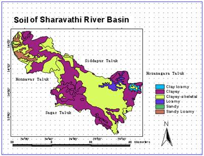
Fig 6.6: Soil of Sharavathi river basin
Lithological Distribution: The Sharavathi river basin belt is made up of various types of Schist, chiefly chloritic and in places micaceous or hornblendic, associated with volcanic rocks of different types. Along with them are found some highly altered sedimentary rocks such as quartzite, conglomerates, limestone, shale and banded ironstones (ferruginous quartzite). The factors of Lithology, which affect the occurrence of landslide, are:
- Occurrence of fine-grained materials such as shale and unconsolidated alluvium.
- Distribution of slope angles within a geological unit’s outcrop area, affecting the susceptibility ranking of each unit.
- Rocks rich in clay (montmorillonite, bentonite), mica, calcite, gypsum etc., which are promoters of weathering.
- Geological structures i.e. occurrence of inclined bedding planes, joints, fault or shear zone are the planes of weakness, which create conditions of instability.
Undercutting along the hill slopes for laying roads or rail tracks can result in instability. Some parts of Uttar Kannada belong to an older group of sediments and intrusives, all very highly metamorphosed with a group of plutonic intrusive, is collectively termed as the peninsula gneiss. A capping of laterite, which is locally the source of iron, manganese ores and ocher, frequently overlies both. In detail the main types of rocks, which exist in the Sharavathi river basin area, are
- Metamorphic rocks: These rocks are formed through the operation of various metamorphic processes on the pre-existing rocks involving either textural, structural or change in mineralogical composition. Metamorphic rocks are classified on the basis of texture of structure, degree of metamorphism, mineralogical composition and mode of origin.
The main rocks of this type are:
- Migmatites and granodiorite: Characterised as banded rocks consisting of alternating layers of quartz and feldspar of high metamorphic grade. They are banded or striped rocks with alternating layers of dark and light minerals. The dark layers commonly contain biotite, and the light layers commonly contain quartz and feldspar. Shale is the usual parent rock of gneiss. Granite is the parent rock of some gneiss.
- Greywacke / argillite- is a severely hardened sandstone with mica and feldspar, sometimes containing fossils.
- Meta grey wake argillite is a mudstone, hardened by pressure.
- Amphibolitic metapelitic schist/ pelitic schist, calc-silicate rock - are foliated medium-grade metamorphic rocks with parallel layers, vertical to the direction of compaction.
- Quartz chlorite schist with orthoquartzite: metamorphic rock containing abundant obvious micas several millimetres across. Shale is the parent rock of schist.
- Quartzite: represents metamorphosed sandstone with its interlocking grains of quartz. The rock fractures through the grains (rather than between the grains as it does in sandstone). The parent rock is quartz sandstone.
- Plutonic rocks: These are coarse-grained igneous rocks formed at considerable depths, generally between 7-10 km below the surface of earth where there is a very slow rate of cooling.
The main rocks under this are:
- Grey Granite - Granitic rock is much less common on the surfaces of other planets; a fact having to do with the fractionation (where early crystallising minerals separate from the rest of magma), a process that takes place uniquely on earth, due to the prevalence of plate tectonics.
- Residual Capping and Unconsolidated sediments: It is the insoluble products of rock weathering, which have escaped erosion by geological agents and still cover the rock from which they have been derived.
The main rocks under this are: Laterite; Alluvium / beach sand, alluvial soil.
- Volcanic / Meta volcanic: These are igneous rocks formed by the cooling and crystallisation of lava erupted from volcanoes on the surface of the earth.
The main rocks under these are:
- Metabasalt and tuff - (sometimes called greenstone if massive and green, or green schist if foliated and green) - the green colour comes from chlorite (soft and bluish green) and epidotic (pea green). The parent rock is basalt. The grade of metamorphism is very low.
- Metabasalt including thin ironstone.
- Meta basalt thin subardinate metarhyalite and associated metabasic intrusives.
- Amphibolitic metapelitic schist/ pelitic schist, calc-silicate rock: Abundant amphibole is present; may be lineated and subjected to higher temperatures and pressures than Metabasalt, greenstone, or green schist.
Since in the study area the type of rocks are diverse and need to be evaluated precisely, comparative study table for various types of rocks are prepared and the Lithological distribution map was prepared by digitising the geological toposheet, the map is detailed in Table 6.5 and Figure 6.7.
Table 6.5: Comparative study table for various types of rocks
| Rock |
Compressive strength |
Range of toughness |
Abrasive hardness |
Absorption by wt % |
Porosity% |
Weight kn/m3 |
| Igneous |
34475 to 413700 |
7 to 28 |
37 to 98 |
0.07 to 0.30 |
0.4 to 3.84 |
25.45 to 27.02 |
| Sedimentary |
34475 to 137900 |
2 to 35 |
2 to 26 |
3 to 12 |
1.9 to 27.3 |
18.70 to 26.39 |
| Metamorphic |
110320 to 310275 |
5 to 30 |
6 to 42 |
0.10 to 2.00 |
1.5 to 2.9 |
25.92 to 26.71 |
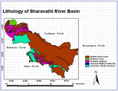
Fig 6.7: Lithology of Sharavathi river basin
Structural Geological Analysis – Lineaments: Where the discontinuity geometry permits sub vertical blocks to be separated from the rock mass through the jointing, movement towards the free face is common. Even where the dip of the base plane (bedding) is less than the natural slope, movement can still occur either by sliding due to the nature of the underlying material or by toppling if the sub vertical joints are opened. A rock plane failure occurs when a set of discontinuities lies parallel to the slope with an angle equal or lower than that of the natural slope. Their influence extends for some 3–5 m on either side of the fracture itself where they appear as a fragmented rock surface in the adjacent area or sheared/ crushed material at the intersection of two such lineaments. This disturbed material assists water infiltration, the lubrication of potential slide planes and the development of pore water pressures. The highest incidence of land sliding can be intercepted in areas where such a linear pattern is interpreted from satellite data in the form of lineaments as shown in Figure 6.8.
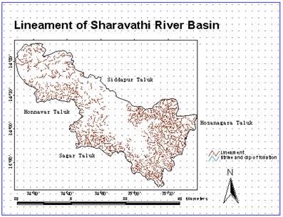
Fig 6.8: Lineament of Sharavathi river basin
Drainage - Sub Basin Analysis: Drainage characterisation is an important factor, which reflects the slope evolution of an area with an indication of the mass wasting and related erosional aspects. Zones with the parallel pattern of drainage associated with strong slope control are the most probable situations for mass movements/ landslides. Drainage is often a crucial measure due to the important role played by pore-water pressure in reducing shear strength. Because of its high stabilisation efficiency in relation to cost, drainage of surface water and groundwater is the most widely used, and generally the most successful stabilisation method. Deep drains that are trenches sunk into the ground to intersect the shear surface, extending below it achieve drainage of the failure surfaces. The drainage in the area is mainly dendritic drainage consisting of a network of channels resembling tree branches. The study area is divided into 16 sub-basins on the basis of major tributaries and existing drainages as shown in Figure 6.10. Areas underlain by nearly horizontal sedimentary rocks and some areas of igneous and metamorphic rocks commonly display dendritic drainage, where tributaries join larger channels at various angles as shown in Figure 6.9, the drainage map of the study area. Table 6.6 shown below gives the details of the sub basins’ soil type and lithology.
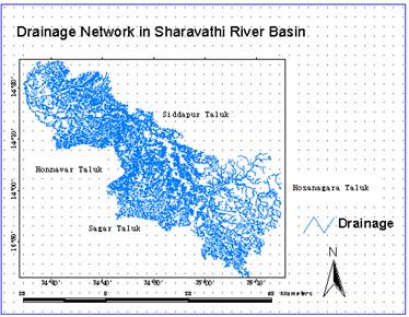
Fig 6.9: Drainage network in Sharavathi river basin
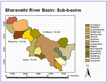
Fig 6.10: Sharavathi river basin: Sub-basins
Table 6.6: Sub-basin details
| Sub Basin |
Name |
Soil Type |
Lithology |
| DS1 |
Chandavar |
Clayey, Clayey skeletal, Sandy loamy |
Metamorphic rocks, Plutonic rocks |
| DS2 |
Haddinabal |
Clayey, Clayey skeletal, Sandy loamy |
Volcanic / Meta volcanic, Metamorphic rocks |
| DS3 |
Magod |
Clayey, Clayey skeletal, Sandy loamy |
Volcanic / Meta volcanic, Residual capping |
| DS4 |
Dabbefall |
Clayey, Clayey skeletal |
Metamorphic rocks, Volcanic / Meta volcanic |
| DS5 |
Mavinagundi |
Clayey, Clayey skeletal |
Metamorphic rocks, Residual capping |
| DS6 |
Kattlekan |
Clayey, Clayey skeletal |
Metamorphic rocks, Residual capping |
| DS7 |
Gudankateholé
|
Sandy, Sandy loamy, Clayey skeletal |
Metamorphic rocks, Unconsolidated sediments |
| US1 |
Nandiholé |
Clayey, Clayey skeletal, loamy |
Metamorphic rocks |
| US2 |
Haridravathi |
Clayey, Clayey skeletal, loamy, clay loamy |
Metamorphic rocks |
| US3 |
Mavinaholé |
Clayey skeletal |
Metamorphic rocks |
| US4 |
Sharavathi |
Clayey, Clayey skeletal |
Metamorphic rocks, Volcanic / Meta volcanic |
| US5 |
Yenneholé |
Clayey, Clayey skeletal |
Metamorphic rocks, Residual capping |
| US6 |
Hurliholé |
Clayey |
Metamorphic rocks, Residual capping |
| US7 |
Nagodiholé |
Clayey, Clayey skeletal |
Metamorphic rocks, Residual capping |
| US8 |
Hilkunji |
Clayey, Clayey skeletal |
Metamorphic rocks |
| US9 |
Linganamakki |
Clayey, Clayey skeletal, loamy |
Metamorphic rocks, Volcanic / Meta volcanic |
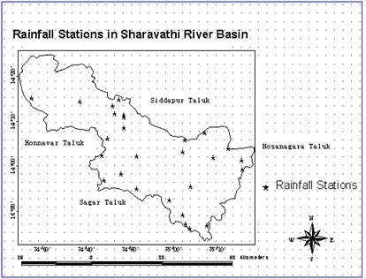
Rainfall Analysis: The Sharavathi river basin area receives high rainfall of more than 3000 mm and landslides occur when a high intensity rain follows a prolonged steady rainy season. This normally occurs during the middle phase of southwest monsoon or if the pre-monsoon is high in the initial phase in the month of August or September. A short duration of intense rainfall can be used to predict the likelihood of a landslide. It increases the groundwater level through either short, intense precipitation or prolonged rainfall of lower intensity. The monthly variations of rainfall at all the stations were evaluated to see the intensity of rainfall. For this, the average and standard deviation was calculated as shown in Figures 6.11. Rainfall exceeding 200 mm/day has been found to initiate catastrophic landslides in the Western Ghats area. The data in Table 6.7 of 21 years of 27 locations in the study area is considered as a base layer preparation theme for landslide analysis. The average rainfall data of the locations along with the map generated are shown in Figures 6.12 and 6.13.
Fig 6.11: Monthly variation of rainfall in sub-basins
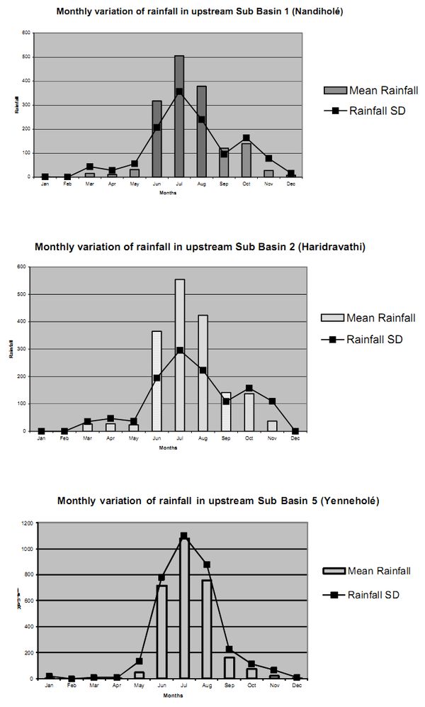
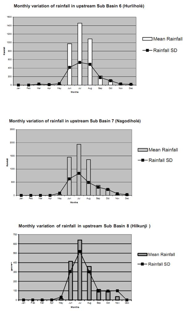
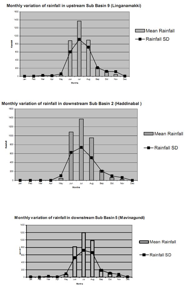
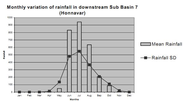
Table 6.7: Rainfall averages of sub-basin stations
| Sub Basin |
Rainfall Station |
Average |
Std. Dev |
Cumm. Average |
Cumm. Std. Dev |
| US1 |
Anandapuram |
1706.58571 |
461.5981 |
1503.35 |
±798.78 |
| Battemallappa |
1546.09524 |
1137.395 |
| Ulloru |
1257.39524 |
797.3731 |
| US2 |
Rippanapate |
1347.44762 |
482.459 |
1675.03 |
±689.81 |
| Arasalu |
2002.61905 |
689.8127 |
| US5 |
Aralagodu |
4682.65714 |
1070.998 |
2830.85 |
±1035.64 |
| Kogar |
6219.98095 |
1143.34 |
| Kaarani |
276.195238 |
1265.686 |
| Biligaaru |
144.585714 |
662.575 |
| US6 |
Byakodu |
4324.89524 |
1160.166 |
3879.40 |
±937.66 |
| Tumari |
3433.91429 |
715.1738 |
| US7 |
Nagodi |
5693.6 |
1279.73 |
5693.6 |
±1279.73 |
| US8 |
Koduru |
1638.92857 |
1115.03 |
1638.92 |
±1115.02 |
| US9 |
Genasinakuni |
1584.7 |
1014.937 |
3546.39 |
±1455.87 |
| Sagar |
1730.0381 |
638.4296 |
| Nagara |
4801.25238 |
1075.84 |
| Chakranagar |
5378.65238 |
1570.547 |
| Nilskal |
4850.47619 |
2863.244 |
| Mattikai |
3669.78095 |
2097.127 |
| Hosanagara |
2809.87619 |
931.0309 |
| DS2 |
Gerusoppa |
3736.32857 |
1825.549 |
3736.32 |
±1825.54 |
| DS5 |
Mavinagundi |
263.195238 |
1206.112 |
3374.87 |
±872.26 |
| Linganamakki |
3436.99048 |
552.7307 |
| Kargal |
4144.32381 |
891.2878 |
| Talakalale |
4116.33333 |
598.9735 |
| A.B. Site |
4913.51429 |
1112.203 |
| DS7 |
Honnavar |
2736.60476 |
1418.18 |
2736.60 |
±1418.18 |
Fig 6.12: Graphical representation of rainfall averages
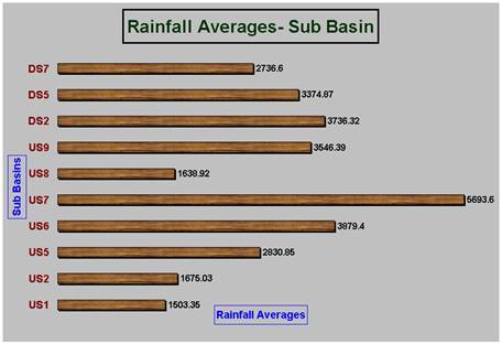
Fig 6.13: Rainfall stations in Sharavathi river basin
7. REMOTE SENSING DATA ANALYSIS
Land Cover Analysis - Computation of Normalised Difference Vegetation Indices (NDVI)
Land cover analysis was done using Normalised Difference Vegetation Index (NDVI) that helps in identifying observed physical cover including vegetation (natural or planted) and has an ability to minimise topographic effects while producing a linear measurement scale. NDVI has been computed depending on the extent of the vegetation in a region for the land cover analysis. This is mainly for regions with good vegetation i.e. western and southeast part of the study area where soil reflection is very less because of dense canopy covers.
NDVI is mainly based on the combinations of visible red and near infrared bands and are widely used to generate vegetation Indices. It was computed based on data grabbed by space borne sensors in the range 0.6-0.7 (red band) and 0.7-0.9 (NIR band), which help in delineating vegetation and non-vegetation areas. It is an index derived from reflectance measurements in the red and infrared portions of the electromagnetic spectrum to describe the relative amount of green biomass from one area to the next. The values, which are seen range from –1 to 1, where non-existence is shown at –1 and existence is shown at 1. The values indicate both the status and abundance of green vegetation cover and biomass. This is computed using the algorithm of
NDVI = (IR-R) / (IR+R)
It is generally seen that:
- High near-infrared reflectance and low visible reflectance yield high values in vegetated areas.
- Features like water and clouds yield negative index values since they have larger visible reflectance than near-infrared reflectance.
- Vegetation indices are seen near zero for rock and bare soil areas since they have similar reflectance in the two bands.
The NDVI image generated for the study area is shown in Figure 7.1 below.
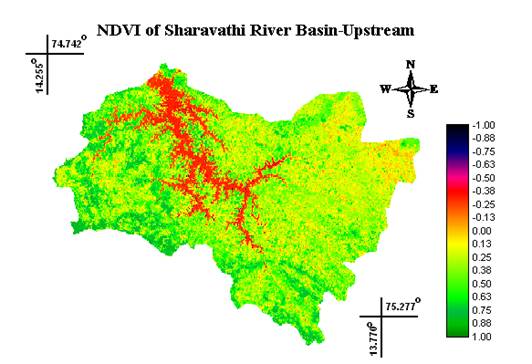
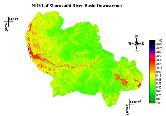
Fig 7.1: NDVI of Sharavathi river basin
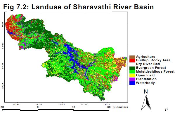
Land Use Analysis - Supervised Classification
- Data used: IRS 1D LISS III – MSS Data was used for land cover, land use analyses. Satellite imageries of Path 97 - Row 63, provide the entire image of Sharavathi catchment region. LISS (corresponding to 0.5-0.6, 0.6-0.7, 0.7-0.9 mm of electromagnetic spectrum or Green, Red and NIR bands) sensor data was used for the analysis.
- Geometric correction: The existing bands were geometrically corrected taking the known points’ latitude and longitude values from the image and the existing accurate corresponding ground values existing in Survey of India toposheets and Ground Control Points taken from field using GPS. Resampling of the images was done considering the polynomial model because it uses polynomial coefficients to map between image spaces. The projection for raw satellite imagery used was UTM and to do that, first order polynomial is normally good and was taken. The GCP tool references for images were taken from toposheets. The image obtained after this was re-sampled with these points to get the correct image.
- Field data: Field data, which was uniformly distributed all over the basin, was collected using GPS over the entire basin so as to represent all land use categories . This helped in considering all spectral classes constituting each information class for adequate representation in the training set statistics used to classify an image. The test areas are taken as prototype of representative areas and they are located during the training stage of supervised classification by intentionally designating more training areas than that which was actually needed to develop the classification statistics.
- Vegetation classification: Data regarding trees were noted down in quadrants of 20 x 20 m2, which mainly contain trees species; density and canopy cover along with the GPS value.
Supervised classification requires more input and experience by the analyst but it can produce more accurate and useful results than unsupervised classification. The strategy is to identify homogenous, representative samples of the different land cover types of interest. These samples are called training areas. The selection of appropriate training areas is based on the analyst's familiarity with the area and it is ideally supported by reliable ancillary sources, such as aerial photos, maps, or other ground truth data. The spectral information in all spectral bands for the pixels comprising these training areas is used to recognise spectrally similar areas for each class. The computer uses a special algorithm (of which there are several variations) to determine "the spectral signatures” for each training class, although there are a number of different algorithms available for performing supervised classification. If the classification is accurate, the resulting classes represent the categories within the data that the user originally identified. Thus, in a supervised classification we are first identifying the information classes, which are then used to determine the spectral classes, which represent them. In supervised training, it is important to have a set of desired classes in mind, and then create the appropriate signatures from the data. The various types of algorithms, which are used in supervised classification, include: Maximum likelihood, Mahalanobis distance and minimum distance. Maximum likelihood decision rule is based on the probability that a pixel belongs to a particular class. The basic equation assumes that these probabilities are equal for all classes, and that the input bands have normal distributions.
- Maximum likelihood supervised classifier: In comparison with various classification algorithms, maximum likelihood classification approach has higher accuracy. Maximum likelihood classification is a supervised classification for which training sites were selected and sufficient training data and Ground Control Points (GCP) were used. Accurate mapping or inventory of natural resources requires ground control points (GCP), which are necessary to fit details extracted from satellite images. Based on the training data collected in the field, remote sensing data was classified in the land use pattern of built up areas (open rocky area, buildings, etc.), evergreen to semi evergreen forest, moist deciduous forest, plantation (acacia + areca), agricultural areas, open area (barren area, open uncultivated agriculture land, dry grasslands, dry river bed, etc.) and waterbodies.
- Accuracy assessment: The overall objective of the training process is to assemble a set of statistics that describe the spectral response pattern for each land cover type to be classified in an image. Two of the most commonly employed approaches are as follows.
- Homogeneous test areas selected by the analyst.
- Test pixels or areas selected randomly.
This requires substantial reference data and a thorough knowledge of the geographic area. Most importantly, the quality of the training process determines the success of the classification stage and, therefore, the value of the information generated from the classification. The recognising pixel that represents the classes that has been extracted is shown in Figure 7.2 below.
8. LANDSLIDE PRONE ZONE MAPPING
In order to do landslide prone zone mapping, suitable map layers along with attribute tables were considered necessary for inclusion in the GIS. Giving relative weightages of susceptibility to the classified objects of these maps, weights’ map is prepared that also incorporated image processing techniques. Weight value for landslide susceptibility is calculated from the landslide density of each class of each control factor category. This helped in the division of the entire study area in various zones of hazard classes as per the weight assigned for various classes. The various layers, which were finally used for assigning weights for ranking, are as follows.
- Slope
- Aspect
- Landuse/ Landcover
- N.D.V.I image i.e. vegetation
- Geology i.e. Lithological distribution
- Soil characteristics
- Drainage density
- Lineament density
- Road density
- Rainfall intensity
The parameters are prioritised based on the hazard potential i.e. higher the ranking higher is the area prone to landslide. The study area is divided into zones of landslide vulnerability viz., very high, high, very moderate, moderate, poor and very poor. The landslide magnitude definition says that the rankings, which are given to various factors, are.
- Rank 1 (Very Poor): No damage to infrastructure because of low-lying areas.
- Rank 2 (Poor): Injury, burial or death of people is likely.
- Rank 3 (Very Moderate): Destruction of smaller trees, powerlines, damage to houses possible, and removal of roadways are likely.
- Rank 4 (Moderate): Destruction of large trees, and burial of small houses possible.
- Rank 5(High): Destruction of large infrastructure, and derailment of trains likely.
- Rank 6(Very High): Destruction and burial to multiple infrastructures, parts of towns and villages.
Ranking of Study Area based on Slope, Land Use, and other GIS Database
The study area is ranked on various parameters discussed earlier considering the sub basin clusters as a base and weights are calculated on the ranking basis, which is as follows:
- Slope: The slope map of the study area was derived from the contours and Digital elevation model, as explained in the methodology. The slopes of the study area are defined at an interval of 10 degrees as shown in Figure 8.1 below.
Fig 8.1: Slope -Sharavathi river basin
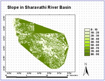
Slope is a very important parameter in any landslide hazard zonation mapping. In the study area slope varies from 0 to 60 degrees. If the slope is higher, then there is a chance of occurrence of landslide. The final ranking is done on the basis of the amount of existence of high sloping in a cluster and weight values are given to slope parameters using Table 8.1 and map was prepared.
Table 8.1: Criteria for ranking terrain based on Slope
| Sr. No |
Slope value |
Rank |
| 1 |
0-10° |
1 |
| 2 |
10-20° |
2 |
| 3 |
20-30° |
3 |
| 4 |
30-40° |
4 |
| 5 |
40-50° |
5 |
| 6 |
>50° |
6 |
As the terrain is undulating, each sub basin has heterogeneous slopes. Hence, the cumulative weights were calculated based on the share of each slope range in a cluster for each sub basin. The final ranking was computed based on cumulative weights as listed in Table 8.2. Based on this, the slope-ranking map for the river basin was generated and is given in Figure 8.2.
Table 8.2: Cumulative weights of Slope
| Cumulative Values |
Weights |
| 1-1.2 |
1 |
| 1.2-1.4 |
2 |
| 1.4-1.6 |
3 |
| 1.6-1.8 |
4 |
| 1.8-2.5 |
5 |
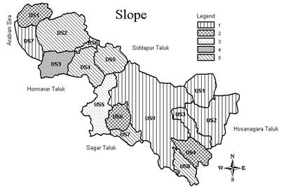
Fig 8.2: Ranking based on Slope
- Aspect: The aspect is the direction in which the maximum slope exists. This is used to determine the direction of downhill faces in the line of steepest descent. Aspects are output in decimal degrees and use standard azimuth designations from north. In regions where the surface is perfectly flat with slope = 0, aspect is assigned a value of flat terrain. All the sides of the slope were assigned the value of its present existence, which is shown in Figure 8.3 below.
Fig 8.3: Aspect of Sharavathi river basin
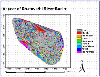
Aspect is also one of the important phenomena, which alters the existence of landslide. To monitor this, as the southwest area is having sea and wind blowing from that side, which could affect landslide generation, aspect map was prepared as shown in Figure 8.4 and map was created taking the ranking values shown in Table 8.3.
Table 8.3: Criteria for ranking terrain based on Aspect
| Sr. No |
Aspect |
Rank |
| 1 |
North or East |
1 |
| 2 |
North West |
2 |
| 3 |
West |
3 |
| 4 |
South East |
4 |
| 5 |
South |
5 |
| 6 |
South west |
6 |
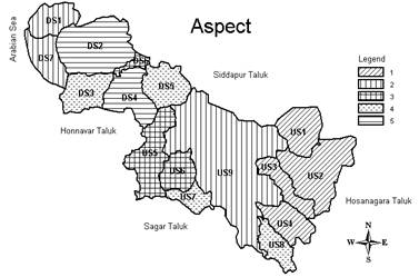
Fig 8.4: Ranking based on Aspect
- Landuse/ Landcover: The remote sensing data (MSS data) of the study area was classified by supervised classification approach using maximum likelihood classifier. The types of classification falling in various sub basins on the basis of their area existing in that was used to calculate the susceptibility for landslide. The ranks given in Table 8.4 were used and maps generated for the same is shown in Figure 8.5.
Table 8.4: Criteria for ranking based on Land use
| Sr. No |
Landuse type |
Rank |
| 1 |
Built up |
1 |
| 2 |
Water |
2 |
| 3 |
Evergreen forest |
3 |
| 4 |
Moist deciduous forest |
4 |
| 5 |
Plantation |
5 |
| 6 |
Agriculture |
6 |
| 7 |
Open area |
7 |
Classified image indicate that each sub-basin has different level / extent of land use. Hence, based on the extent of each type and on ranking for each category, a composite ranking is derived for each sub-basin as given in the Table 8.5 below. This takes into account susceptibility for landslide by each category and its spread in each sub-basin.
Table 8.5: Cumulative weights of Land use
| Cumulative Values |
Weights |
| 3.25 - 3.5 |
1 |
| 3.5 - 3.75 |
2 |
| 3.75 - 4.0 |
3 |
| 4.0 - 4.25 |
4 |
| 4.25 - 4.5 |
5 |
| 4.5 - 5.0 |
6 |
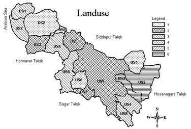
Fig 8.5: Ranking based on Land use
- N.D.V.I image: N.D.V.I was computed for the study area reflecting the amount of vegetation lying in a particular sub basin. NDVI values normally range from –1 to +1. Values greater than 0 show vegetation and the range indicate extent of canopy cover / vegetation in the region. Higher values reflect good canopy cover or good vegetation. The amount and extent of each range of NDVI for each sub basin was evaluated using their value given in Table 8.6 and depicted pictorially in Figure 8.6.
Table 8.6: Criteria for ranking terrain based on NDVI ranges
| Sr. No |
Vegetation range |
Rank |
| 1 |
> -0.4 |
5 |
| 2 |
-0.4 to 0 |
4 |
| 3 |
0 to 0.2 |
3 |
| 4 |
0.2 to 0.4 |
2 |
| 5 |
> 0.4 |
1 |
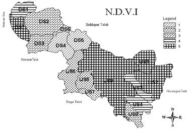
Fig 8.6: Ranking based on NDVI
- Lithological distribution: An important aspect is the existence of rocks, for instance, when the underlying bedrock is porous due to the presence of sandstone or some volcanic-formed rock, it drains faster. Impermeable bedrock, such as granite, keeps water in the soil. Over the time, excess water is transferred down to the water table or to stream channels, and some is stored for future use by plants. Bedrock type can also determine slide potential. Some rocks, such as shale and volcanic-formed rocks weather to form sticky clay soils. Sandstones, granites, and micas wear down into coarse porous soils that are easily moved. In the study area, the existing rock types are classified on their various properties with the rank ranging 4-5 due to lot of lineaments crack, water content, thin soft week beds. The existing landslide is also taken into consideration to decide the stability of the existing rocks. For the hardened rocks, which rank lowly, i.e. 3, it is mainly due to existing of major river and dam areas with lots of water percolation and seepage. The area with laterite also faces mining and excavation, which loosens that rock type. And lastly for high ranking i.e. 2 and 1, the factors considered are high weathering, high permeability, and presence of unconsolidated and weak material in lesser quantity. Existence of Metabasalt or basalt is mainly due to its hardness with less weathering and no seepage of water due to absence of layering. The rankings are shown in Table 8.7.
Table 8.7: Criteria for ranking based on Lithology
| Sr. No |
Lithology |
Rank |
| 1 |
Amphibolitic metapelitic schist/ pelitic schist, calc-silicate rock |
4 |
| 2 |
Greywacke / argillite |
4 |
| 3 |
Meta grey wake argillite |
4 |
| 4 |
Quartz chlorite schist with orthoquartzite |
4 |
| 5 |
Laterite |
3 |
| 6 |
Migmatites and granodiorite - tonalitic gneiss |
3 |
| 7 |
Grey granite |
2 |
| 8 |
Meta basalt thin subardinate metarhyalite & assosiated metabasic intrusives |
2 |
| 9 |
Metabasalt & tuff |
2 |
| 10 |
Metabasalt including thin iron stone |
2 |
| 11 |
Quartzite |
2 |
| 12 |
Alluvium / beach sand, alluvial soil |
1 |
Investigation of lithology of the Sharavathi river basin shows that each sub basin has heterogeneous lithological features. In view of this, depending on share of lithological features in each sub basin, a composite ranking is derived based on weighted averages as shown in Table 8.8 and the map is given in Figure 8.7.
Table 8.8: Cumulative weights of Lithology
| Cumulative Values |
Weights |
| 2.0-2.50 |
1 |
| 2.50-3.0 |
2 |
| 3.0-3.5 |
3 |
| 3.5-4.0 |
4 |
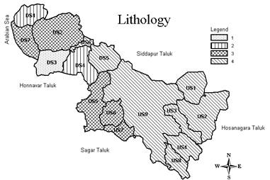
Fig 8.7: Ranking based on Lithology
- Soil types: In the study area, occurrence of landslide is mainly found due to the presence of huge thickness of loose soils when mixed with water near the Sharavathi river area. As discussed earlier, the ranking is mainly done keeping the water holding capacity, bulk density, porosity and permeability of the soil in concern. The area of a certain soil falling in a sub basin with other soils helps in determining the prone area of the sub basin for landslide. The ranking Table 8.9 and map generated for the same in Figure 8.8 are as follows.
Table 8.9: Criteria for ranking terrain based on Soil
| Sr. No |
Soil |
Rank |
| 1 |
Clayey |
6 |
| 2 |
Clay loamy |
5 |
| 3 |
Clayey-skeletal |
4 |
| 4 |
Loamy |
3 |
| 5 |
Sandy loamy |
2 |
| 6 |
Sandy |
1 |
Cumulative values were evaluated through the relevance of the lithological map as soil types vary with the type in cluster so the percentage area was calculated for various types to calculate the weights for the map as is shown in Table 8.10.
Table 8.10: Cumulative weights of Soil
| Cumulative Values |
Weights |
| 2.5-3.0 |
1 |
| 3.0-3.5 |
2 |
| 3.5-4.0 |
3 |
| 4.0-4.5 |
4 |
| 4.5-5.0 |
5 |
| 5.0-6.0 |
6 |
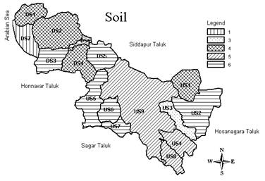
Fig 8.8: Ranking based on Soil
- Drainage density: In the study area, as discussed, the drainage is mainly dendritic, where the density was computed by using the area in square kilometre of individual sub basins and number of drains falling in that area. This is mainly done to see the dependence of the type of drain on the involvement of water in percolation. The first order drains have various aspects in their drainage with respect to the third order due to lesser water flow and percolation. The drainage density also decides the susceptibility for landslides. The ranking shown in Table 8.11, which was considered in making the map for drainage density as shown in Figure 8.9, is as follows.
Table 8.11: Criteria for ranking based on Drainage density
| Sr. No |
Drainage density |
Rank |
| 1 |
0-1.0 |
1 |
| 2 |
1.0-2.0 |
2 |
| 3 |
2.0-3.0 |
3 |
| 4 |
3.0-4.0 |
4 |
| 5 |
4.0-5.0 |
5 |
| 6 |
>5.0 |
6 |
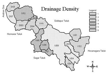
Fig 8.9: Ranking based on Drainage density
- Lineament density: As discussed earlier, the influence of landslide lies on 3–5 m on either side of the fracture itself where they appear as a fragmented rock surface in the adjacent area or sheared/crushed material at the intersection of two such lineaments. To evaluate the amount of effects the lineaments impart on landslide, the density was calculated similar to the calculation of drainage density. The ranking criteria based on the density are given in Table 8.12 and the same for each sub basin is shown pictorially in Figure 8.10.
Table 8.12: Criteria for ranking based on Lineament density
| Sr. No |
Lineament density |
Rank |
| 1 |
0-0.25 |
1 |
| 2 |
0.25-0.5 |
2 |
| 3 |
0.5-0.75 |
3 |
| 4 |
0.75-1.0 |
4 |
| 5 |
1.0-1.25 |
5 |
| 6 |
1.25-1.50 |
6 |
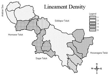
Fig 8.10: Ranking based on Lineament density
- Road density: The areas close to the existing roads in an undulating terrain are more prone for landslide as they are built across the toe of hills and have removed the support. The criteria tables for ranking, which was used, and map generated are shown in Table 8.13 and Figure 8.11 respectively.
Table 8.13: Criteria for ranking terrain based on Road density
| Sr. No |
Road density |
Rank |
| 1 |
0-0.25 |
1 |
| 2 |
0.25-0.5 |
2 |
| 3 |
0.5-0.75 |
3 |
| 4 |
0.75-1.0 |
4 |
| 5 |
1.0-1.25 |
5 |
| 6 |
1.25-1.50 |
6 |
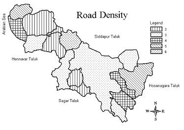
Fig 8.11: Ranking based on Road density
- Rainfall: The relationship between rainfall and landslides aids in the understanding of the landslide processes and also provides a basis for predicting widespread slope failures. Heavy antecedent rainfall or a short duration of intense rainfall triggers most of the landslides. The ranking as shown in Table 8.14 and the map 8.12 created on the basis of amount of rainfall occurred at 27 locations in various sub basins is as follows.
Table 8.14: Criteria for ranking terrain based on Rainfall
| Sr. No |
Rainfall |
Rank |
| 1 |
0-2000 mm |
1 |
| 2 |
2000-3000 mm |
2 |
| 3 |
3000-3500 mm |
3 |
| 4 |
3500-3750 mm |
4 |
| 5 |
>3750 mm |
5 |
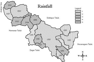
Fig 8.12: Ranking based on rainfall
Resultant Layers Creation- Overlaying
In order to map landslide susceptibility zones in the river basin, considering various causal factors discussed so far, a composite map is generated in GIS by overlaying all causal factor-ranking layers. Higher weights indicate the sub-basin’s susceptibility for landslides. Percentage share of each sub basin’s weights is computed and are given in the Table 8.15. Values greater than 65.353 % or cumulative weights of 32.6765 were considered to confer the sub-basins’ susceptibility to landslides.
Table 8.15: Final ranking values of factors in all Sub-basins
| Sub-basin |
Aspect |
NDVI |
Drainage |
Landuse |
Lineament |
Road |
Lithology |
Slope |
Soil |
Rain |
Sum |
% Share |
| DS7 |
2 |
5 |
2 |
3.76 |
2 |
4 |
3.12 |
1.12 |
2.95 |
2 |
27.95 |
55.9 |
| US1 |
1 |
5 |
1 |
4.15 |
5 |
3 |
4 |
1.05 |
4.5 |
1 |
29.70 |
59.4 |
| US9 |
2 |
5 |
2 |
3.7 |
2 |
3 |
3.75 |
1.15 |
4.7 |
4 |
31.30 |
62.6 |
| US3 |
1 |
4 |
2 |
4.62 |
5 |
4 |
4 |
1.1 |
4 |
2 |
31.72 |
63.44 |
| US5 |
3 |
2 |
4 |
3.94 |
3 |
3 |
3.25 |
1.47 |
5.6 |
2 |
31.26 |
63.44 |
| DS1 |
2 |
4 |
3 |
3.79 |
2 |
5 |
2.69 |
1.32 |
4.5 |
3 |
31.30 |
62.6 |
| DS6 |
3 |
1 |
5 |
3.44 |
1 |
2 |
3.52 |
1.99 |
5.4 |
4 |
30.35 |
60.7 |
| US2 |
1 |
5 |
1 |
4.93 |
5 |
5 |
4 |
1.05 |
5.3 |
1 |
33.28 |
66.56 |
| US4 |
1 |
4 |
2 |
4.39 |
6 |
4 |
3.66 |
1.2 |
5 |
3 |
34.25 |
68.5 |
| DS3 |
4 |
3 |
5 |
3.57 |
3 |
3 |
2.05 |
1.77 |
5.1 |
3 |
33.49 |
66.98 |
| US6 |
3 |
2 |
4 |
4.12 |
3 |
2 |
3.32 |
1.37 |
6 |
5 |
33.81 |
67.62 |
| DS2 |
5 |
3 |
5 |
4.15 |
2 |
2 |
3.16 |
1.97 |
4.2 |
4 |
34.48 |
68.96 |
| US7 |
4 |
2 |
4 |
3.68 |
5 |
2 |
3.18 |
1.9 |
5.8 |
5 |
36.56 |
73.12 |
| US8 |
4 |
3 |
3 |
3.98 |
6 |
3 |
4 |
2 |
5 |
1 |
34.98 |
69.96 |
| DS4 |
5 |
1 |
6 |
3.97 |
3 |
2 |
2.94 |
1.97 |
4.2 |
3 |
33.08 |
66.16 |
| DS5 |
4 |
1 |
5 |
3.57 |
1 |
6 |
3.98 |
2.1 |
5.2 |
3 |
34.85 |
69.7 |
| |
|
|
|
|
|
|
|
|
|
|
|
|
| Ranks Assigned |
5 |
5 |
6 |
5 |
6 |
6 |
4 |
2 |
6 |
5 |
50.00 |
|
| |
Maximum |
73.12 |
| |
Minimum |
55.9 |
| |
Average |
65.353 |
The sub basins were grouped into landslide susceptibility zones on the basis of their weights of all causal factors. The zones prone for landslide are classified into 6 zones from very high to very poor based on the relative share of causal factors. Within susceptible sub-basins, considering slope and aspect, data regions were identified that are prone to landslides. This was also compared with the field data of existing landslides. The landslide prone zones with regions of higher susceptibility are depicted in Figure 8.13.

Data Analysis
In order to understand the role of various causal factors on landslide in a region, parametric analysis was carried out. Field data of landslides is overlaid on the landslide zonation map as shown in Figure 8.14, and corresponding attribute values for the respective field points were derived from the map and listed in Table 8.16.
Regression analysis of each causal factors (as independent variable) and landslide proneness as dependent variable did not reveal any significant relationship (at p < 0.05). In order to understand cumulative effects, stepwise regression was carried out and the probable relationship is given by:
LS= -1.05801- (0.345238797) S + (0.204210801) L + (0.646266454) RD + (0.615561311) L D – (0.089156743) DD + (0.07793196) R +(1.888490458) A - (1.49700461) Sl – (0.00015434) Lu – (0.296976094) N
R = correlation coefficient = 0.5948, standard error of y estimate= 1.008
Where dependent causal factors are: LS= Landslide Susceptibility, S= Soil, L=Lithology, RD= Road Density, LD= Lineament Density, DD= Drainage Density, R= Rainfall, A= Aspect, Sl= Slope, Lu= Landuse and N= NDVI.
Table 8.16: Ranking of landslide variables for analysis
| Landslide |
Landslide Group |
Soil |
Lithology |
Road density |
Lineament density |
Drainage density |
Rainfall |
Aspect |
Slope |
Landuse |
NDVI |
| 1 |
4 |
2 |
3 |
5 |
2 |
3 |
3 |
2 |
2 |
7 |
3 |
| 2 |
3 |
2 |
3 |
5 |
2 |
3 |
3 |
2 |
2 |
1 |
3 |
| 3 |
4 |
4 |
3 |
5 |
2 |
3 |
3 |
2 |
2 |
6 |
3 |
| 4 |
3 |
4 |
3 |
5 |
2 |
3 |
3 |
2 |
2 |
5 |
2 |
| 5 |
3 |
4 |
4 |
4 |
2 |
2 |
2 |
2 |
1 |
6 |
3 |
| 6 |
5 |
4 |
4 |
4 |
2 |
2 |
2 |
2 |
1 |
1 |
3 |
| 7 |
5 |
4 |
4 |
4 |
2 |
2 |
2 |
2 |
1 |
7 |
3 |
| 8 |
3 |
4 |
1 |
4 |
2 |
2 |
2 |
2 |
1 |
1 |
3 |
| 9 |
3 |
4 |
1 |
4 |
2 |
2 |
2 |
2 |
1 |
1 |
3 |
| 10 |
3 |
4 |
1 |
4 |
2 |
2 |
2 |
2 |
1 |
5 |
3 |
| 11 |
3 |
2 |
3 |
4 |
2 |
2 |
2 |
2 |
1 |
6 |
3 |
| 12 |
3 |
2 |
3 |
4 |
2 |
2 |
2 |
2 |
1 |
6 |
4 |
| 13 |
4 |
2 |
3 |
4 |
2 |
2 |
2 |
2 |
1 |
7 |
2 |
| 14 |
2 |
2 |
2 |
3 |
3 |
5 |
3 |
4 |
4 |
7 |
2 |
| 15 |
1 |
4 |
2 |
3 |
3 |
5 |
3 |
4 |
4 |
1 |
3 |
| 16 |
3 |
4 |
4 |
2 |
2 |
5 |
4 |
5 |
5 |
1 |
2 |
| 17 |
2 |
4 |
4 |
2 |
2 |
5 |
4 |
5 |
5 |
5 |
1 |
| 18 |
2 |
4 |
4 |
2 |
2 |
5 |
4 |
5 |
5 |
5 |
1 |
| 19 |
1 |
6 |
4 |
6 |
1 |
5 |
3 |
4 |
5 |
3 |
1 |
| 20 |
5 |
4 |
2 |
2 |
3 |
6 |
3 |
5 |
5 |
3 |
1 |
| 21 |
3 |
4 |
4 |
2 |
3 |
6 |
3 |
5 |
5 |
3 |
1 |
| 22 |
1 |
6 |
4 |
6 |
1 |
5 |
3 |
4 |
5 |
4 |
2 |
| 23 |
2 |
6 |
4 |
6 |
1 |
5 |
3 |
4 |
5 |
5 |
1 |
| 24 |
3 |
4 |
4 |
3 |
3 |
4 |
2 |
3 |
3 |
4 |
2 |
| 25 |
2 |
6 |
4 |
2 |
3 |
4 |
4 |
3 |
2 |
4 |
3 |
| 26 |
3 |
6 |
4 |
2 |
3 |
4 |
4 |
3 |
2 |
4 |
3 |
| 27 |
2 |
6 |
2 |
2 |
3 |
4 |
4 |
3 |
2 |
3 |
2 |
| 28 |
2 |
6 |
4 |
3 |
2 |
2 |
4 |
2 |
1 |
1 |
2 |
| 29 |
3 |
6 |
4 |
3 |
2 |
2 |
4 |
2 |
1 |
1 |
2 |
| 30 |
3 |
6 |
4 |
3 |
2 |
2 |
4 |
2 |
1 |
3 |
2 |
| 31 |
2 |
6 |
4 |
3 |
2 |
2 |
4 |
2 |
1 |
5 |
2 |
| 32 |
5 |
4 |
4 |
3 |
2 |
2 |
4 |
2 |
1 |
5 |
3 |
| 33 |
2 |
4 |
4 |
3 |
2 |
2 |
4 |
2 |
1 |
1 |
3 |
| 34 |
2 |
6 |
4 |
2 |
5 |
4 |
5 |
4 |
5 |
4 |
2 |
| 35 |
1 |
6 |
4 |
2 |
5 |
4 |
5 |
4 |
5 |
7 |
3 |
| 36 |
2 |
6 |
4 |
3 |
2 |
2 |
4 |
2 |
1 |
4 |
2 |
| 37 |
1 |
4 |
4 |
3 |
3 |
4 |
2 |
3 |
3 |
4 |
2 |

Socio-Economic Analysis of Highly Sensitive Landslide Areas
Landslide tampers the landscape and disturbs the habitats of flora and fauna. It severely degrades the environment and declines the quality of life for many people. Landslides have incapacitating effect on the economy and generally the people in the lower economic strata are affected the most, as they are economically ill and cannot cope with the disruption of life due to this natural hazard. Socio-economic survey was carried out while doing the field survey for existing landslide areas and the problems people face due to landslides were enumerated after evaluating the landslide prone areas as per the village boundary and population of 1991 census. The villages with the population that would be affected due to landslide are shown in Table 8.17. Proper remedial/corrective measures and preventive actions can be implemented at this stage so that impact can be minimised and distortions due to this are less and controllable.
Table 8.17: Village and population affected due to landslides
| SR. NO |
VILLAGE NAME |
AREA IN HECTARE |
TOTAL POPULATION |
POPULATION DENSITY
NO / HECTARE |
PER CAPITA AGRICULTURE LAND IN HECTARE |
| 1 |
PAVINKURVE |
183.32 |
1031 |
5.62 |
0.06 |
| 2 |
KARKI |
1149.18 |
5429 |
4.72 |
0.05 |
| 3 |
MALLAPUR |
56.75 |
261 |
4.60 |
0.60 |
| 4 |
CHANDAVAR |
2134.16 |
2881 |
1.35 |
0.02 |
| 5 |
HOSAKULI |
574.19 |
2767 |
4.82 |
0.01 |
| 6 |
DUGGUR |
142.67 |
297 |
2.08 |
0.21 |
| 7 |
KADLE |
822.11 |
1605 |
1.95 |
0.04 |
| 8 |
NILKOD |
688.04 |
806 |
1.17 |
0.28 |
| 9 |
VANDOOR |
375.23 |
925 |
2.47 |
0.41 |
| 10 |
MAVINKURVE |
657.54 |
3335 |
5.07 |
0.00 |
| 11 |
HADINBAL |
383.57 |
2156 |
5.62 |
0.06 |
| 12 |
MUTTA |
244.12 |
1065 |
4.36 |
0.07 |
| 13 |
GUNDABALA |
937.86 |
1112 |
1.19 |
0.03 |
| 14 |
JANKADKAL |
3374.11 |
731 |
0.22 |
0.18 |
| 15 |
SARALGI |
685.29 |
1285 |
1.88 |
0.26 |
| 16 |
HULEGAR |
565.39 |
362 |
0.64 |
0.01 |
| 17 |
KASARKOD |
391.23 |
6719 |
17.17 |
0.00 |
| 18 |
NAGODI |
2566.83 |
1963 |
0.76 |
0.10 |
| 19 |
VARAMBALLI |
422.48 |
456 |
1.08 |
0.27 |
| 20 |
DEVARASALIKE |
68.58 |
45 |
0.66 |
0.26 |
| 21 |
KALLUVIDIABBIGALLA |
1252.34 |
447 |
0.36 |
0.18 |
| 22 |
BILLODI |
352.01 |
320 |
0.91 |
0.34 |
| 23 |
TOGARE |
1199.65 |
623 |
0.52 |
0.21 |
| 24 |
HONNEBYLU |
1106.56 |
934 |
0.84 |
0.22 |
| 25 |
ANEGADDE |
359.46 |
235 |
0.65 |
0.25 |
| 26 |
SONALE |
931.19 |
1064 |
1.14 |
0.24 |
| 27 |
ADAVALLI |
115.77 |
90 |
0.78 |
0.32 |
| 28 |
KOLAGI |
628.16 |
459 |
0.73 |
0.27 |
| 29 |
KODASE |
865.90 |
248 |
0.29 |
0.27 |
| 30 |
SAVANTHUR |
671.66 |
569 |
0.85 |
0.24 |
| 31 |
RYAVE |
1572.41 |
702 |
0.45 |
0.22 |
| 32 |
HILUKUNGI |
930.98 |
323 |
0.35 |
0.14 |
| 33 |
HIRIYOGI |
181.66 |
245 |
1.35 |
0.19 |
| 34 |
THNNIVE |
842.77 |
893 |
1.06 |
0.15 |
| 35 |
RAMACHANDRAPURA |
489.93 |
606 |
1.24 |
0.13 |
| 36 |
NELLUNDE |
210.38 |
159 |
0.76 |
0.09 |
| 37 |
BELUR |
1716.26 |
662 |
0.39 |
0.22 |
| 38 |
MUMBARU |
1054.58 |
1122 |
1.06 |
0.21 |
| 39 |
URALAGALLU |
3194.56 |
118 |
0.04 |
0.82 |
| 40 |
KANURU |
1702.84 |
275 |
0.16 |
0.24 |
| 41 |
KANAPAGARU |
3056.32 |
659 |
0.22 |
0.24 |
| 42 |
MARATI |
2100.86 |
784 |
0.37 |
0.19 |
| 43 |
VALUR |
1035.03 |
165 |
0.16 |
1.25 |
| 44 |
ADAGALALE |
960.35 |
424 |
0.44 |
0.32 |
| 45 |
KODANAVALLI |
2448.55 |
782 |
0.32 |
0.17 |
| 46 |
MARUTHIPURA |
787.68 |
765 |
0.97 |
0.12 |
| 47 |
KODUR |
844.5 |
1296 |
1.50 |
0.01 |
| 48 |
HIREMAITHE |
802.99 |
635 |
0.79 |
0.02 |
| 49 |
ALAVALI |
1211.99 |
683 |
0.563 |
0.06 |
After evaluating the socio economic aspects, the following points were evaluated for the study area:
- 51518 persons reside in the areas/villages, which are prone to landslides.
- The 12 villages having higher average density of population can be affected more due to this natural hazard, and the average population density is 1.841.
- Total area of villages falling under landslide prone zone is 490 square kilometres.
- Among all the villages, 64 % of area falls in forest and the remaining 36% is the area where the people reside in and use for their needs.
- In the villages, per capita agriculture land on an average is 0.22, which reflects the vital role played by agriculture in their lives.
- Some existing landslide occurrences is due to anthropogenic activities i.e. diversion of streams for increase of agriculture area or for better irrigation.
- Total literacy in the area is roughly around 55%.
- Since the literacy rate is high, it is important to tell them about the hazardous impacts and how they can be avoided.
RESULTS AND DISCUSSION
The landslide prone zone mapping of Sharavathi river basin reveals that sub basins, namely, Haddinabal (DS2), Magod (DS3), Dabbefall (DS4), Mavinagundi (DS5), Haridravathi (US2), Sharavathi (US4), Hurliholé (US6), Nagodiholé (US7) and Hilkunji (US8) show higher probability of landslide occurrence, mainly due to the following aspects:
- Heavy rain in particular months would cause enough erosive force to erode significant bank areas along meanders (which have relatively poor vegetation cover) and trigger highly prone slope failures.
- The establishment of reservoirs has ushered a change in the flow regime of the streams, leading to higher susceptibility for slope failures and consequent damages in the downstream of the Sharavathi river basin.
- With the inherent fragility of the terrain, the slides may occur due to high precipitation and the existence of reservoirs, which enhance the pore-water pressure beyond the threshold limits.
- Sub basins, which are found prone to landslide, are in undulating terrains.
- Laterite, which is locally the source of iron and manganese ores and ocher, lie in all the downstream and coastal areas and is generally extracted for mining and construction use. These disturbed laterite slopes may slide as the prone areas have abundance of this Lithological unit.
- The sub basins in the study area, which are identified as prone are having close proximity of lineaments that render some areas more vulnerable to hazards.
- Slopes are high in the identified sub basins and may fail if disturbed, i.e. highly prone for landslides due to any human disturbance that is likely to affect the equilibrium.
- It is seen clearly that the study area is having an abundance of road network and due to it’s the presence of hilly terrain, new tracks are being laid to reduce the discomfort of circuitous routes. These creations of new tracks in hilly area or through mountains have led to imbalances in the terrain.
- In addition to these, anthropogenic activities like diversion of streams, encroachment of valley for areca plantations and agriculture are aggravating landslide proneness.
Remedial Measures
This hazard can be avoided through implementing protective measures considering delicately positioned properties of the study area as follows:
- To minimise any future slope failure the construction of the road should be at a properly planned position and haphazard road constructions must be avoided.
- Planting vegetation or maintaining slope terraces can also reduce slope-runoff so regulating the amount of vegetation clearing reduces the risk of increasing the number of landslide-prone areas.
- In view of recurring danger to life and property, an appropriate management strategy should be adopted to prevent diversion of streams, deforestation, conversion of hilly areas for plantation and agricultural activities. This would minimise landslides and mass failures.
- Construction of establishments without considering past or estimated peak flow stages may cause extensive damage to property that can be avoided by proper planning.
- Any disturbance that would contribute to deforestation must be avoided. This may fail slope in an above normal monsoon year.
- Socio economic survey reveals that the literacy rate is high in the area and the local residents must be made aware of the consequences of landslide hazards and the causal factors that aggravate the situation due to unplanned anthropogenic activities.
CONCLUSION
As per the landslide prone zone mapping, slides may occur due to infiltration of water in the unconsolidated material due to reservoirs and toe cutting of the hilly area for developmental activities.
The study area with heavy rainfall of more than 4500 mm and instances of high intensity rainfall, which not only increases the surface flow in river basin but also induces a high piezometric head in the unsorted colluvium of clayey soil and metamorphic rocks. The area of study is having an abundance of wet surface due to heavy rainfall and surface water. The stability of the wet surface further reduces because of the existence of clayey soil due to its low porosity and permeability. Geological existence of metamorphic rocks along the lineament features increases hydrostatic pressures on the existing unconsolidated material, which trigger down slope movement.
In the study area it is found that the slope excavation is mainly done in order to develop residential sites or build roads on sloping terrain as the area is having completely forested hilly terrain full and as a result now some slopes are much steeper than the pre-existing natural slopes. The added weight of fill placed on slopes can also result in an area prone for landslide hazards. Small landslides are common along roads, in either the road cut or the road fill. During the field visit it was found that most of the existing landslides are near the roads. Road associated landslides are good indicators of the potential impacts of excavation on new construction.
REFERENCES
- Abhishankar, K (1975) Gazetteer of India, Karnataka state gazetteer, Shimoga district, Government of Karnataka Publication, Bangalore
- Akgun A, Serhat Dag S, and Bulut F (2007) Landslide susceptibility mapping for a landslide-prone area (Findikli, NE of Turkey) by likelihood-frequency ratio and weighted linear combination models. Environ Geol. doi:10.1007/s00254-007-0882-8
- Alca´ntara-Ayala, I., 2002. Geomorphology, natural hazards, vulnerability and prevention of natural disasters in developing countries. Geomorphology 47 (2–4), 107– 124.
- Anbalagan R, 1992. Landslide hazard evaluation and zonation mapping in mountainous terrain. Eng Geol 32, pp. 269–277.
- Atkinson, P.M., Massari, R., 1998. Generalized linear modelling of landslide susceptibility in the central Apennines, Italy. Computers & Geosciences 24, 373– 385.
- Bernard W.P and Trent D.D, 2001. Geology and the Environment, Brooks/Cole, Pacific Grove, USA. pp.269
- Cannon, S.H., 2000. Debris flow response of southern California watersheds burned by wildfire. In: Wieczorec, G.F., Naeser, N.D. (Eds.), Debris Flow Hazards Mitigation: Mechanics, Prediction and Assessment. Balkema, Rotterdam, pp. 45– 52.
- Clerici A, Perego S, Tellini C, Vescovi P (2002) A procedure for landslide susceptibility zonation by the conditional analysis method. Geomorphology 48:349–364.
- Cooke R., Doornkamp,J., 1990.Geomorphology in Environmental Management: A New Introduction, Oxford Univ. Press, Oxford.
- D. O'Leary, J. Friedman and H. Pohn, 1976. Lineament, linear, lineation: some proposed new standards for old terms, Geological Society of America Bulletin 87, pp. 1463–1469
- Dai, F.C., Lee, C.F., 2001. Terrain-based mapping of landslide susceptibility using a geographical information system: a case study. Canadian Geotechnical Journal 38, 911 – 923.
- Das, B.K. (1981) District census handbook: Shimoga district, Census of India 1981 series 9: Karnataka Government Press, Bangalore.
- Das, B.K. (1981) District census handbook: Uttara Kannada district, Census of India 1981 series 9: Karnataka Government Press, Bangalore.
- David F. Maune (2001) Digital elevation model technologies and applications: the DTM users manual, ASPRS, Maryland
- Derruau M., 1983. Geomorfologia, Ariel Geografia, Barcelona.
- Donati L, Turrini MC (2002) An objective method to rank the importance of the factors predisposing to landslides with the GIS methodology: application to an area of the Apennines (Valnerina; Perugia, Italy). Eng Geol 63:277–289.
- Fausto Guzzetti (2005), Probabilistic landslide hazard assessment at the basin, doi:10.1016/j.geomorph.2005.06.002
- Garcı´a-Ruiz, J.M., Arna´ez, J., Ortigosa, L., Go´mez Villar, A., 1988.Debris flows subsequent to a forest fire in the Najerilla River Valley (Iberian System, Spain). Pirineos 131, pp.3– 24.
- Giacomo D’Amato Avanzi, Roberto Giannecchini, Alberto Puccinelli., 2004. The influence of the geological and geomorphological settings on shallow landslides. An example in a temperate climate environment: the June 19, 1996 event in northwestern
- Gómez H., Kavzoglu T., 2005. Assessment of shallow landslide susceptibility using artificial neural networks in Jabonosa River Basin, Venezuela, Eng Geol 78, pp-11-27.
- Greenbaum, D., Tutton, M., Bowker, M., Browne, T., Buleka, J., Greally, K., Kuna, G., McDonald, A., Marsh, S., O'Connor, E., Tragheim, D., 1995. Rapid Methods of Landslide Hazard Mapping: Papua New Guinea Case Study. British Geological Survey. Technical Report WC/95/27.
- Greenway, D.R., 1987. “Vegetation and Slope Stability.” SlopeStability, John Wiley & Sons Ltd., pp.187 - 230.
- Gupta, R.P, 2002 Remote Sensing Geology, 2nd edition, Springer-Verlag, Heidelberg. pp. 445.
- Guzzetti F., Reichenbach P., Cardinali M., Galli M., Ardizzone F., (2005), Probabilistic landslide hazard assessment at the basin scale, doi:10.1016/ j.geomorph.2005.06.002
- H. Chen and C. F. Lee, A dynamic model for rainfall-induced landslides on natural slopes, Geomorphology, Volume 51, Issue 4, 25 April 2003, Pages 269-288
- Hutchinson JN (1995) Landslide hazard assessment. In: Proc VI Int Symp on Landslides, Christchurch, 1 : 1805–1842
- Jibson WR, Edwin LH, John AM (2000) A method for producing digital frequency seismic landslide hazard maps. Eng Geol 58:271–289.
- Jiu J.J., Xu-Sheng, W., Subhas N., 2005, Confined groundwater zone and slope instability in weathered igneous rocks in Hong Kong, Engineering Geology 80 pp.71-92
- Kamat, S.U. (1985) Gazetteer of India, Karnataka state gazetteer, Uttara Kannada district, Government of Karnataka Publication, Bangalore
- Kesavulu C.N, 1997. Textbook of Engineering geology, Macmillan India Limited, New Delhi.
- Lee S, Choi J, Min K (2004a) Frequency landslide hazard mapping using GIS and remote sensing data at Boun, Korea. Inter J Remote Sens 25(11):2037–2052.
- Lee S, Choi U (2003) Development of GIS based geological hazard information system and its application for landslide analysis in Korea. Geosci J 7:243–252.
- Lee S, Chwae U, Min K (2002) Landslide susceptibility mapping by correlation between topography and geological structure: the Janghung area, Korea. Geomorphology 46:49–162.
- Lee S, Min K (2001) Statistical analysis of landslide susceptibility at Yongin, Korea. Environ Geol 40:1095–1113
- Lee S, Pradhan B (2006) Landslide hazard assessment at Cameron Highland Malaysia using frequency ratio and logistic regression models. Geophy Res Abstracts, 8:SRef-ID:1607–7962/gra/ EGU06-A-03241.
- Lee S, Pradhan B (2007) Landslide hazard mapping at Selangor, Malaysia using frequency ratio and logistic regression models. Landslides 4(1):33–41
- Luzi L, Pergalani F, Terlien MTJ (2000) Slope vulnerability to earthquakes at sub-regional scale, using frequency techniques and geographic information systems. Eng Geol 58:313–336.
- McDermid G. and Franklin S., 1995.Remote sensing and geomorphometric discrimination of slope processes, Zeitschrift für Geomorphologie 101, pp.165–185.
- Mohammad Israil and A. K. Pachauri (2003) Geophysical characterization of a landslide site in the Himalayan foothill region, Journal of Asian Earth Sciences
- Nagarajan R, Khire MV (1998) Debris slides of Varandh ghat, west coast of India. Bull Eng Geol Environ 57: 59–63
- Nagarajan, R., A. Roy, R. Vinodkumar, A. Mukherjee, & M.V. Khire (2000), Landslide hazard susceptibility mapping based on terrain and climatic factors for tropical monsoon regions. Bull Eng. Geol. Env. (2000) 58
- Pachauri AK, Pant M (1992) Landslide hazard mapping based on geological attributes. Eng Geol 32: 81–100
- Piyoosh Rautela and Ramesh Chandra Lakhera (2000) Landslide risk analysis between Giri and Tons Rivers in Himachal Himalaya (India), JAG l Volume 2 – Issue 3/4
- R. Anbalagan, (1992), Landslide hazard evaluation and zonation mapping in mountainous terrain. Engineering Geology, 32 (1992) 269-277
- Radhakrishna B.P., Vidyanadhan R. (1994) Geology of Karnataka, Geological Society of India, Bangalore.
- Reed W, James S.M, 2002.Essentials of Geology, 3rd edition, Brooks/Cole, Pacific Grove, USA. pp.269.
- S.K. Paul, S.K. Bartarya, Piyoosh Rautela, A.K. Mahajan (2000) Catastrophic mass movement of 1998 monsoons at Malpa in Kali Valley, Kumaun Himalaya India, Geomorphology 35 2000: 169–180
- Selby M., 1993. Hillslope Materials and Processes, Oxford Univ. Press, Oxford.
- Shiva Prasad, et al. Soils of Karnataka for optimizing landuse, National Bureau of Soil survey and Landuse Planning, Nagpur
- Squier, L.R., Harvey, A.F., 2000. Two debris flows in Coast Range, Oregon, USA: logging and public policy impacts. In: Wieczorec, G.F., Naeser, N.D. (Eds.), Debris Flow Hazards Mitigation: Mechanics, Prediction and Assessment. Balkema, Rotterdam, pp- 127– 138.
- Terzaghi, K., Peck, R.B., 1967. Soil Mechanics in Engineering Practice. John Wiley and Sons, New York. p. 432
- Tuscany (Italy), Eng Geol 73, pp. 215–228
- Varnes, 1984; landslide hazard zonation: a review of principles and practices. UNESCO, Paris, pp.1-63.
- Vijith H., Madhu G., 2007,Estimating potential landslide sites of an upland sub-watershed in Western Ghat’s of Kerala (India) through frequency ratio and GIS, Environ Geol.doi:10.1007/s00254-007-1090-2.
- Wu, W., Sidle, R.C., 1995. A distributed slope stability model for steep forested basins. Water Resources Research 31, 2097– 2110.
- Zezere JL, Reis E, Garcia R, Oliveira S, Rodrigues ML, Vieira G, Ferreira AB (2004) Integration of spatial and temporal data for the definition of different landslide hazard scenarios in the area north of Lisbon (Portugal). Natural Haz Earth Sys Sciences 4:133–146.
- http://www.gisdevelopment.net/application/natural_hazards/landslides/nhls0013pf.htm
- http://www.gisdevelopment.net/application/natural_hazards/landslides/nhls0010pf.htm
- http://www.gisdevelopment.net/application/natural_hazards/landslides/nhls0011pf.htm
- http://www.cnr.colostate.edu/~denis/pubs_online/Litschert_and_Dean_2000.PDF
- http://www.gisdevelopment.net/application/natural_hazards/landslides/mi03128.htm
- http://www.gisdevelopment.net/application/natural_hazards/landslides/mi03040.htm
- http://www.gisdevelopment.net/application/natural_hazards/landslides/nhls0012.htm
- http://www.geospatialtoday.com/articles/article_4.asp
- http://www.gisdevelopment.net/application/natural_hazards/landslides/nhls0005.htm
- http://www.gisdevelopment.net/application/natural_hazards/landslides/nhls0006.htm
- http://www.gisdevelopment.net/aars/acrs/1994/ts3/ts3004.shtml
- http://www.gisdevelopment.net/aars/acrs/1997/ps3/ps3006.shtml
- http://www.gisdevelopment.net/aars/acrs/1996/ts3/ts3003.shtml
- http://www.gisdevelopment.net/aars/acrs/2000/ts12/laus0010.shtml
- http://www.gisdevelopment.net/application/natural_hazards/landslides/mi03098abs.htm
- http://dionysos.gssr.sk/ig_home/exchange/ppaudits/p2002_Praha(Handlova,Paudits-Bednarik).pdf
BIBLIOGRAPHY
- Drury, S.A. (1987) Image interpretation in geology, Allen and Unwin, London
- Prost, Gary L. (2001) Remote sensing for geologists: a guide to image interpretation, 2nd Gordon and Breach Science Publishers, Australia
- Lillesand, Thomas M.; Kiefer, Ralph W. (2002) Remote sensing and image interpretation, 4th John Wiley & Sons, Inc., New York
- Majumdar, S.P., Singh, R.A. (2000) Analysis of soil physical properties, Agro bios, Jodhpur
- Verbyla, David L. (2002) Practical GIS analysis, Taylor & Francis, London
- Prabin Singh (1996) A textbook of engineering and general geology, S.K.Kataria and sons, Delhi.
- Kessavulu channa N. (1997) Textbook of engineering geology, Macmillan India Limited, Delhi.
- Radhakrishna B.P. (1996) Mineral resources of Karnataka, Geological society of India, Bangalore
- http://www.gisdevelopment.net/application/natural_hazards/landslides/nhls0007pf.htm
- http://convention.allacademic.com/aag2003/sessions.html?letter=R
- http://www.gisdevelopment.net/application/natural_hazards/landslides/index.htm
- http://www.onid.orst.edu/~chevallj/GIS.landslides.htm
- http://convention.allacademic.com/aag2003/sessions.html?letter=R
- http://www.gisdevelopment.net/application/natural_hazards/landslides/index.htm
- http://www.onid.orst.edu/~chevallj/GIS.landslides.htm
- http://www.geologyuk.co.uk/downloads/kathmandu_seminar.doc
- http://www.gisdevelopment.net/aars/acrs/1997/ps3/ps3006pf.htm
- http://gisweb.athena.bcit.ca/students/class02-03/gisb009/litreview.htm
- http://www.gisdevelopment.net/aars/acrs/2000/ps1/ps102pf.htm
- http://geosun.sjsu.edu/paula/285/285/eb_sem.htm
- http://rst.gsfc.nasa.gov/Front/tofc.html
- http://www.gisdevelopment.net/aars/acrs/1997/ts3/ts3001pf.htm
- http://www.geogr.muni.cz/lgc/gis98/proceed/PAVELKA.html
- http://www.mysteries-megasite.com/main/bigsearch/landslides.html
- http://staff.aist.go.jp/s.tsuchida/itit/f_report/3odaji.pdf
- http://www.mysteries-megasite.com/main/bigsearch/landslides.html
- http://www.onid.orst.edu/~chevallj/GIS.landslides.htm
- http://moose.cee.usu.edu/sinmap/sinmap_poster.ppt
- http://www.fes.uwaterloo.ca/crs/gp555/gisp.pdf
- http://www.onid.orst.edu/~chevallj/GIS.landslides.htm
- http://staff.aist.go.jp/s.tsuchida/itit/f_report/3odaji.pdf
- http://www.cnr.uidaho.edu/remotesensing/Projects/Landslide_hazard.html
- http://www.mountaingis.org/
- http://www.cnr.uidaho.edu/remotesensing/Projects/Strategic_Research2002/Landslide%20Hazard.htm
- http://www.ceworld.org/ceworld/Presentations/Computing/Rose1.cfm
- http://moose.cee.usu.edu/sinmap/sinmap_poster.ppt
- http://www.ceeraindia.org/cgi-bin/ceera_indown.pl?filename=about.pl
- http://deis158.deis.unibo.it/gis/chapt0.htm
- http://www.geoplace.com/asiapac/2000/0700/0700lnd.asp
- http://www.gisdevelopment.net/proceedings/mapindia/2000/poster/pos001.htm
- http://ag.arizona.edu/classes/rnr271/articles/logic/logic.html
- http://www.gisdevelopment.net/application/natural_hazards/landslides/mi03128pf.htm
- http://www.geovista.psu.edu/sites/geocomp99/Gc99/054/gc_054.htm
- http://www-public.tu-bs.de:8080/~aguenthe/bmbf/bmbf01_eng.html
- http://www.itc.nl/ilwis/applications/application07.asp
- http://www.oas.org/en/cdmp/document/kma/udspub5.htm
- http://www.geohaz.com/kingston.htm
- http://geopubs.wr.usgs.gov/map-mf/mf2378/berkpamph.pdf
- http://csd.unl.edu/csd/illustrations/landslides/landslide.html#1.0
- http://landslides.usgs.gov/html_files/nlic/nlicpub.html
- http://www.cityofseattle.net/projectimpact/pioverview/hazardmapping/landslide.htm
- http://www.adpc.ait.ac.th/audmp/rllw/themes/th1-bandara.pdf
- http://www.oregonshowcase.org/projects/state/downloads/hazard_trg_6_2000/08_landslide.pdf
- http://3d.wr.usgs.gov/docs/wgmt/3d/pp02.html#task5
- http://www.geol.pdx.edu/People/DCP/G424-GIS/metrosld.doc
- http://www.yapirehberi.net/Heyelan.htm
- http://www.saguenay.ggl.ulaval.ca/saguenay/publi/urgeles2.pdf
- http://anaheim-landslide.com/features.htm
- http://pubs.usgs.gov/of/1995/ofr-95-0213/TABLE.HTML#TABLE
- http://www.ce.berkeley.edu/~khazai/Research/Report/index2.html
- http://www.geospatialtoday.com/articles/article_4.asp
- http://ceos.cnes.fr:8100/cdrom-00b2/ceos1/science/gdta/ang/a2an/78.htm
- http://www.toprak.org.tr/isd/can_41.htm#
- http://www.toprak.org.tr/bildiri_can.htm
|
|