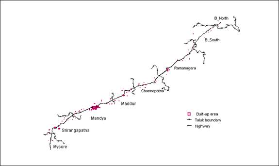
Results and Discussion

The built-up area for 1972 was extracted from the digitized toposheets and is shown in Figure 2. Then villagewise built-up area was computed by overlaying the layer with village boundaries (taluk map with village boundaries) and added to the attribute database for further analyses.

Figure 2: BUILT-UP AREA IN THE BANGALORE – MYSORE SEGMENT IN 1972

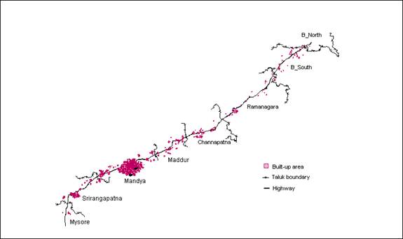
LISS sensor data obtained from the NRSA in three bands, viz., Band 2 (green), Band 3 (red) and Band 4 (near infrared), were used to create a False Colour Composite (FCC). Training polygons (with their co-ordinates) were chosen from the composite image and corresponding attribute data was obtained in the field for these polygons (using GPS). Based on these signatures, corresponding to various land features, image classification was done using Guassian Maximum Likelihood Classifier. From the original classification of land-use of 16 categories the image was reclassified to four broader categories as vegetation, water bodies, open land, and built-up. The built-up theme identified from the image is shown in Figure 3.

Figure 3: BUILT-UP AREA IN THE BANGALORE – MYSORE SEGMENT IN 1998

From the classified image the area under the built-up theme was computed. Area under villagewise built-up theme in the study area was also computed by overlaying a vector layer with village boundaries and tabulated accordingly for further analyses.

Built-up area and Shannon’s entropy
The built-up area computed for temporal data indicated that there was 194% increase in the built-up area from the seventies to late nineties. A more detailed investigation of the distribution of the built-up (Table 2) revealed that the change is higher as the proximity to Bangalore increases. The Bangalore North – South segment had the highest increase in built-up area while it was least in Srirangapatna – Mysore segment with 128%. It can also be observed that there is a declining trend in the change in built-up area as one move from Bangalore towards Mysore.

Table 2: Built-up Area and Shannon’s Entropy for the Study Area

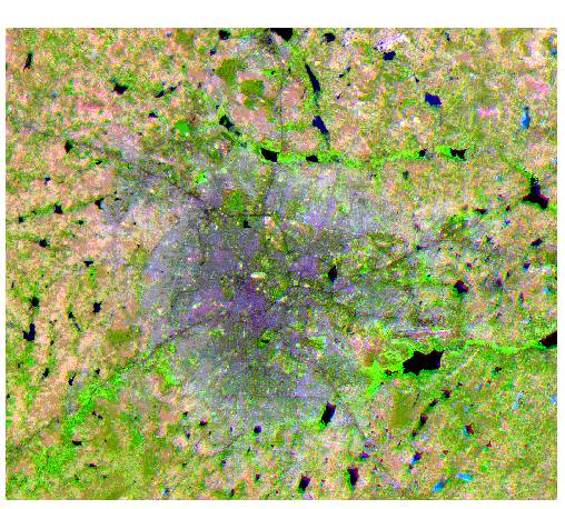
Shannon’s entropy was computed for villagewise built-up area, wherein each village was considered as an individual zone (n = total number of villages). This revealed that the distribution of built-up in the region in 1972 was slightly dispersed than in 1999. However the degree of dispersion has come down marginally and that distribution is less dispersed or there is the less presence of sprawl when the entire stretch is considered. The values obtained ranges from 2.658 (in 1972) to 2.556 (in 1998) and log n for this region is 4.477. These are higher than the half way mark of log n (that is 2.238) and show some degree of dispersion of built-up in the region. This non-uniform dispersed growth along the road connecting Bangalore and Mysore necessitated further detailed investigations for identifying the pockets of higher growth.

Detailed investigation on the phenomenon was done in the next phase by dividing the study area in to segments / zones. The entire segment of Bangalore – Mysore was split in to two as Bangalore – Ramanagaram and Channapatna – Mysore segments. The percentage built-up change and entropy was calculated for these two segments. The Bangalore – Ramanagaram segment had a higher value of percentage built-up change (330%) than the Channapatna – Mysore segment (181%). The entropy values for the Bangalore – Ramanagaram segment ranges from 2.690 (for 1972) to 2.699 (for 1998) while log n for this region is 3.583 suggests similar trend. In the Channapatna – Mysore segment the entropy value ranged from 2.320 (for 1972) to 2.083 (for 1998) and log n is 3.951. This analysis reveals that the distribution is more dispersed in Bangalore – Ramanagaram segment compared to the later.

On further division of the two segments into four to identify where the actual sprawl is occurring; the segments such as, Bangalore North – South, Ramanagaram – Channapatna, Maddur – Mandya and Srirangapatna – Mysore were obtained. From the results of these (Table 2) this clearly indicated that there was more dispersed distribution of built-up in the region closer to Bangalore and this decreased as the proximity to the city increased. The Bangalore North –South taluks had the highest increase in terms of the percentage built-up change and the entropy values also showed that there was more dispersion in this taluk, thus indicating higher sprawl in this region. Higher sprawl due to the proximity of Bangalore is observed till Channapatna – Ramanagaram segment and fades away towards Mandya. It also inferred that in the Mandya – Maddur segment the distribution was slightly compact with radial sprawl. But in the Srirangapatna – Mysore segment the value of entropy showed marginal change in entropy. Here, the degree of sprawl is not as severe as that in case of other segments, but the marginal increase in entropy value certainly indicates the possibility of increasing sprawl due to enhanced economic activities at Mysore.

With the results of the Shannon’s entropy indicating that regions nearer to Bangalore city had more degree of sprawl, it was decided to work out and understand the patterns of growth in the regions surrounding Bangalore city, in all directions. It was seen that Bangalore sprawling in radial direction from the city centre and linear growth is noticed along all five major roads connecting the city - spreading as five arms stretched outwards (Figure 4). The space between the arms or the major roads acts as the sinks for city development. Further, it is seen that the development occurred around the ring roads that connected these major roads.

Figure 4: FCC OF BANGALORE CITY SHOWING RADIAL PATTERN OF GROWTH FROM THE CITY CENTRE AND LINEAR PATTERN ALONG THE HIGHWAYS