Method

Remote sensing data of Landsat series were downloaded and corrections such as geometric, radiometric and scan-line (for ETM+)  were implemented. Methods used in data analysis for landscape dynamics analysis is given in Figure 2. Survey of India (SOI) topo-sheets of 1:50000 and 1:250000 scales were digitised to derive base layers. Data were analysed using  GRASS - open source GIS package (http://ces.iisc.ernet.in/grass). Method adopted in analysing urban dynamics using Landscape metrics is given in Figure 2 and various stages in data analyses are:

1. Geometric Correction:  Ground control points (GCP’s) for geo-rectification and training data for supervised classification of RS data were collected through field investigations using a handheld GPS. Google Earth data (http://earth.google.com) were used during pre and post classification and also for validation. Bands were geo-corrected with the known GCP’s, and projected to geographic latitude-longitude with WGS-84 datum, followed by masking and cropping of the study area. This method is very common and widespread because of its robustness and higher accuracies of classified data (Hester et al., 2008).

2. Supervised classification using Gaussian maximum likelihood Classifier: In supervised classification, the pixel categorisation process is done by specifying the numerical descriptors of the four land use types (urban, vegetation, water and others (eg:-open space)) present in a scene. It involves (i) training, (ii) classification and (iii) output.

3. Accuracy assessment: Accuracy assessments were done with field knowledge, visual interpretation and also referring Google Earth (http://earth.google.com).

4. Direction and region-wise division of the study area: To understand the landscape dynamics at local level including the understanding of drivers of urban growth the study area is divided direction-wise into 8 zones ( North-North-East (NNE), North-East-East (NEE), South-East-East (SEE), South-South-East (SSE), South-South-West (SSW), South-West-West (SWW), North-West-West (NWW), North-North-west (NNW))and each zone is divided into concentric circle of 2 km incrementing radius  as shown in Figure 3. Thus classified image was divided into 13 concentric circles in 8 directions, which were cropped. This provided 104 regions almost corresponding to the city Corporation administration wards . The classified data corresponding to cropped regions were used for further analysis.

5. Computation of percentage built-up area:  Dynamics of urban built up were assessed using temporal data by computing built up (%) for each region (zone-wise, each circle).

6. Computation of Shannon entropy: To quantify the degree of spatial concentration or dispersion, direction-wise Shannon’s Entropy (Yeh and Li, 2001; Lata et al., 2001; Sudhira et al., 2003) were computed. This is useful and effective for differentiating   various levels of  urbanisation and sprawl. Shannon's  entropy  (Hn) can be used to measure the degree of spatial concentration or dispersion of geographical variables among ‘n’ concentric circles and in 8 directions.           



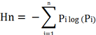
Where, Pi is the proportion of the phenomena occurring in the i^th concentric circle. As per Shannon’s Entropy, if the distribution is maximally concentrated in one circle the lowest value zero will be obtained. Conversely, if it is an even distribution among the concentric circles will be given maximum of log n. This means values closer to zero indicates concentrated growth while values closer to log n indicates the sprawl.

7. Computation of Spatial metrics for each local landscapes: Landscape metrics listed in Table 1 were then computed for 104 regions for each classified image using GRASS (http://wgbis.ces.iisc.ernet.in/foss) and Fragstats  (McGarigal, et al., 2002). However the amount and kind of information that any one metric can offer, or from which information may be inferred may be a limitation and hence a combination of metrics have been used for a more comprehensive understanding of landscape structure and its dynamics (DiBari, J. M., 2007). In this study, 25 landscape metrics were computed and then Principal Component Analysis (PCA) was performed using PAST software and only 11 metrics with higher loadings were selected for further study. PCA is a multivariate analysis that reduces a large number of variables down to a smaller number of relatively independent components associated with a set of specific variables (Tabachnick and Fidell, 2001).

Table 1: Description of metrics used in this study

Sl No.	Indicators	Formula	Description
1.	Built up Area		Total built-up land (in ha)
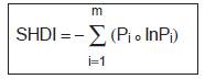
2.	Shannon’s Diversity Index	Where Pi = Proportion of the landscape occupied by patch type (class) i	SHDI  > =0, without limit.
3.	Number of Urban Patches	NPU = n NPU equals the number of urban patches in the landscape.	NPU>0, without limit. It is a fragmentation Index
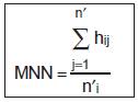
4.	Mean Nearest Neighbor Distance	where h =nearest edge to edge distance n =total no of patches of same type	Mean Nearest Neighbour measures average patch to patch distance. MNN > 0, without limit.
5.	Mean Proximity Index)		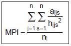The mean proximity index measures the degree of isolation and fragmentation of the corresponding patch type MPI  >=0.
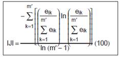
6.	Interspersion and Juxtaposition Index	eik =total length (m) of edge in landscape between patch types (classes) i and k. m =number of patch types (classes) present in the landscape, including the landscape border, if present.	0 < IJI  <=100. IJI approaches 0 when the corresponding patch type is adjacent to only 1 other patch type and the number of patch types increases. IJI = 100 when the corresponding patch type is equally adjacent to all other patch types.
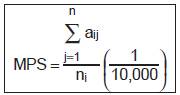
7.	Mean Patch Size	Where aij = Area (m2) of patch ij n =total no of patches of same type	MPS > 0, without limit
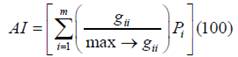
8.	Aggregation index	gii =number of like adjacencies (joins) between pixels of patch type (class) i.max-gii = maximum number of like adjacencies (joins) between pixels of patch type class i based on single count method.Pi= proportion of landscape comprised of patch type (class) i.	1≤AI≤100 AI equals 1 when the patches are maximally disaggregated and equals 100 when the patches are maximally aggregated into a single compact patch
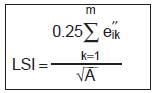
9.	Landscape Shape Index	e″ik Total length (m) of edge in landscape between patch types (classes) I and k; includes the entire landscape boundary and background edge segments, regardless of whether they represent true edge.	Range: LSI ≥ 1, without limit.
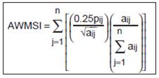
10.	Area weighted mean shape index (AWMSI)	Where   pij =  Perimeter (m) of patch ij	AWMSI = 0 when all patches in the landscape are circular or square. AWMSI = 1, without limit AWMSI increases without limit as the patch shape becomes  irregular
11.	Area weighted Euclidean mean nearest neighbor distance	hij is distance(m) from patch ij to nearest neighboring patch of the same type(class) based on shortest edge to edge distance.	ENN>0, without limit ENN approaches zero as the distance to the nearest neighbor decreases
12.	Mean Shape index	Pij is the perimeter of patch i of type j. aij is the area of patch i of type j.        ni is the total number of patches.      CV (coefficient of variation) equals the standard deviation divided by the mean, multiplied by 100 to convert to a percentage, for the corresponding patch metrics.	It is represented in percentage

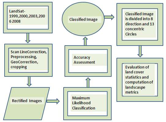
Figure 2: Method adopted for data analysis

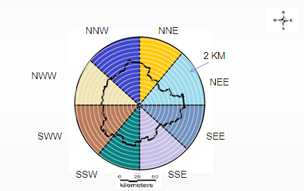
Figure 3: Zones in 8 Directions with concentric circles of 2km incrementing radii