|
EXPERIMENTAL RESULTS AND DISCUSSION
1. Simulated Data
Three images from the 200-bands are shown in Figure 4 and the classified output of the 250 × 250 hyper spectral 200 bands data is shown in Figure 5. The proportions of each of the four minerals were computed based on 10 × 10 groups of pixels for 625 groups [(250 × 250) divided by (10 × 10)].
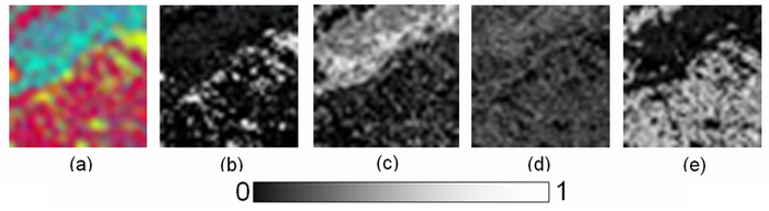
N-FINDR was used to extract the endmembers from the synthetic mixed pixels, which are shown in Figure 6. The endmembers identified by the algorithm (drawn in red) have a good match with the actual ones (green in color). Abundances of each of the minerals from the artificial mixed pixels obtained from LMM are as shown in Figure 7 b-e. Figure 7 a is the 10 times down-sampled image of the original mineral classified image (250 × 250) shown in Figure 5 to compare hard classification with the abundance map visually. A three-layer MLP architecture was made with four input, one hidden and four output layers.
Figure 4. A 200 band hyperspectral image generated from spectral libraries of four different minerals: (a) band 1; (b) band 100; (c) band 200.
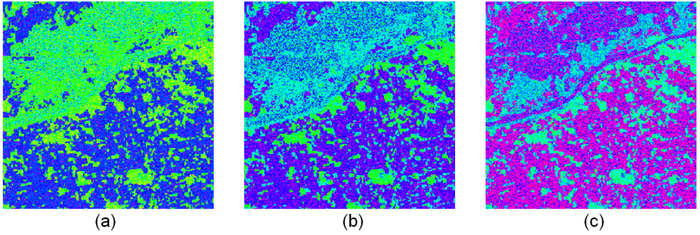
Figure 5. Mineral classified map
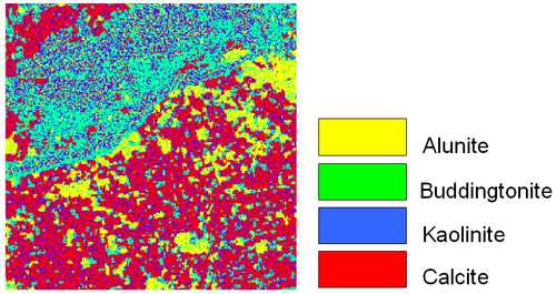
Figure 6. Comparison between the true endmembers and endmembers computed from the N-FINDR algorithm. (X-axis: band number, Y-axis: reflectance value.)
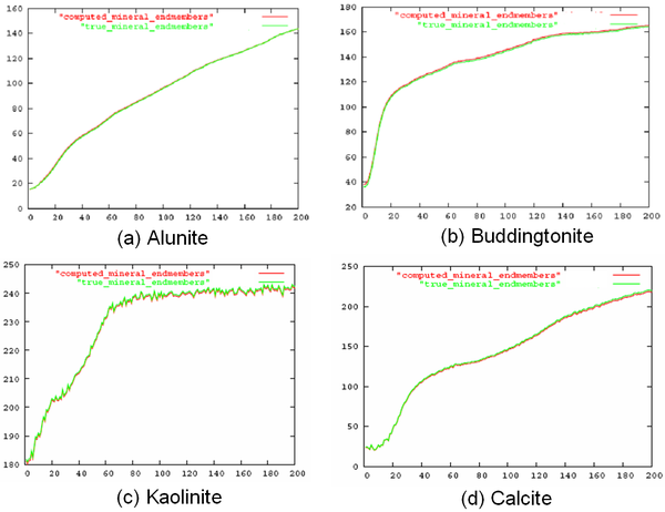
Figure 7. (a) Ten times down-sampled image of the original mineral classified image;
(b)–(e) abundances maps of the four minerals obtained from linear mixture model (LMM).
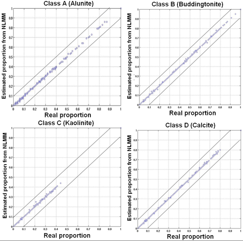
The number of hidden nodes in the hidden layer, learning rate, momentum and epoch were varied in steps to estimate the best abundance values that could account for the non-linearity in the mineral mixtures (as shown in Figure 8), until the performance saturated. Table 1 lists the values of the training parameters along with the training time and the overall RMSE of the MLP network for every 500 epochs. Three measures of performance were used to evaluate the output from artificial dataset—RMSE, correlation, Bivariate Distribution Functions (BDFs). BDF is helpful to visualize the accuracy of prediction by mixture models. BDFs were plotted against the real proportions as shown in Figure 9. Pearson’s product-moment correlation at 95% confidence interval and RMSE between the actual and estimated proportion from LMM and HMM are given in Table 2. The average RMSE of the LMM was 0.0089 ± 0.0022 while the average RMSE of the HMM was 0.0030 ± 0.0001 demonstrating the superiority of the HMM over the LMM. The MLP network can successfully approximate virtually any function when trained correctly.
Figure 8. Abundances maps of the four minerals obtained from HMM
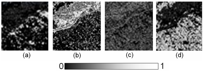
Table 1. Details of training for unmixing of simulated dataset
| No. of epochs |
Learning rate |
Momentum term |
Training time (sec) |
Unmixing
time (sec) |
Overall
RMSE |
| 500 |
0.90 |
0.5 |
4 |
8 |
0.0160 |
| 1000 |
0.85 |
0.4 |
5 |
8 |
0.0117 |
| 1500 |
0.80 |
0.3 |
7 |
7 |
0.0030 |
| 2000 |
0.70 |
0.2 |
7 |
6 |
0.0071 |
| 2500 |
0.60 |
0.1 |
8 |
5 |
0.0115 |
Table 2. Correlation and RMSE between actual and predicted proportions for simulated data
| Classes |
Correlation (r) (p < 2.2e−16) |
RMSE |
| LMM |
HMM |
LMM |
HMM |
| Alunite |
0.67 |
0.97 |
0.0120 |
0.0032 |
| Buddingtonite |
0.71 |
0.98 |
0.0073 |
0.0029 |
| Kaolinite |
0.73 |
0.98 |
0.0088 |
0.0031 |
| Calcite |
0.75 |
0.99 |
0.0076 |
0.0029 |
Figure 9. Bivariate Distribution Functions (BDFs) of simulated test data for the four minerals obtained from HMM.
2. MODIS Data
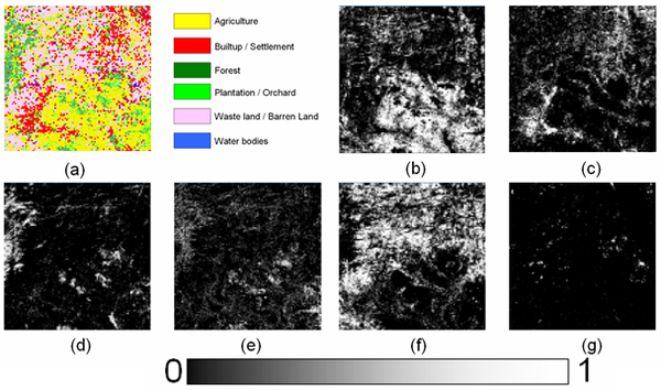
In order to validate the MODIS unmixed image, a LISS-III classified image with an overall accuracy of 95.63% and individual class producers accuracy ranging from 92%–97% and users accuracy ranging from 88%–98% was used. Linear unmixing was applied on MODIS data to obtain the abundance maps. 15% MODIS abundance pixels obtained from LMM were randomly selected to relate with the corresponding LISS-III classified pixels (as ground truth) at the same geographical locations to train the neurons in HMM. MLP architecture with seven inputs (since seven bands of MODIS data were used), one hidden and six output layers (as six different LC classes) was constructed. The MLP based HMM was executed with varied learning rates, momentum and epochs. The momentum term and the learning rate were altered after every 500 epochs. Table 3 lists the values of the training parameters along with the training time and the overall RMSE of the MLP network on the MODIS images after every 500 epochs. The fraction maps obtained from LMM and HMM are shown in Figure 10 b-g and Figure 11 b-g.
Table 3. Details of training for unmixing of MODIS images
| No. of epochs |
Learning rate |
Momentum term |
Training time (sec) |
Unmixing
time (sec) |
Overall
RMSE |
| 500 |
0.90 |
0.05 |
25 |
11 |
0.0220 |
| 1000 |
0.85 |
0.05 |
22 |
11 |
0.0197 |
| 1500 |
0.80 |
0.03 |
22 |
10 |
0.0195 |
| 2000 |
0.70 |
0.02 |
18 |
9 |
0.0191 |
| 2500 |
0.60 |
0.01 |
18 |
8 |
0.0195 |
Figure 10. (a) LISS-III classified map resampled to 100 × 100 pixels. Abundance maps for
(b) agriculture; (c) built-up/settlement; (d) forest; (e) plantation/orchard; (f) wasteland/orchard;
(g) water bodies obtained from LMM.
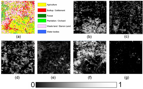
Figure 11. (a)LISS-III classified map resampled to 100 × 100 pixels. Abundance maps for
(b) agriculture; (c) built-up/settlement; (d) forest; (e) plantation/orchard; (f) wasteland/orchard, (g) water bodies obtained from HMM.
BDFs against the real and estimated proportions from MODIS data for LMM and HMM were plotted as shown in Figure 12 and Figure 13 respectively. The Pearson’s product-moment correlation at 95% confidence interval and RMSE between the actual and estimated proportion from LMM and HMM are given in Table 4.
Figure 12. BDFs of MODIS test data from LMM. (a) agriculture; (b) built-up/settlement; (c) forest; (d) plantation/orchard; (e) wasteland/orchard; (f) water bodies.
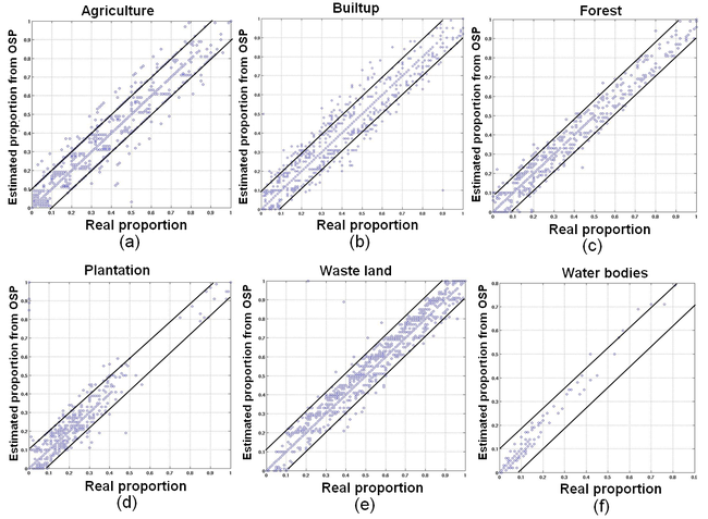
Figure 13. BDFs of MODIS test data from HMM. (a) agriculture; (b) built-up/settlement; (c) forest; (d) plantation/orchard; (e) wasteland/orchard; (f) water bodies.
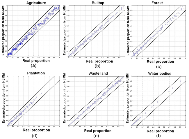
Table 4. Correlation and RMSE between real/reference and predicted proportions for MODIS data.
| Classes |
Correlation (r) (p < 2.2e−16) |
RMSE |
| LMM |
HMM |
LMM |
HMM |
| Agriculture |
0.6730 |
0.9110 |
0.0518 |
0.0271 |
| Builtup/Settlement |
0.6390 |
0.9345 |
1.0519 |
0.0083 |
| Forest |
0.7310 |
0.9411 |
0.0257 |
0.0062 |
| Plantation/Orchard |
0.6990 |
0.9447 |
0.0280 |
0.0061 |
| Waste/Barren land |
0.6599 |
0.9342 |
0.0431 |
0.0073 |
| Water bodies |
0.7799 |
0.9855 |
0.0061 |
0.0016 |
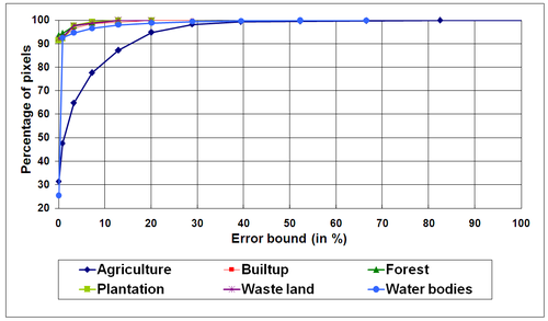
The 100 × 100 pixels from both LMM (Figure 14) and HMM (Figure 15) abundance maps were subjected to error distribution graphs to get a general idea of the range and magnitude of the errors (absolute values of the prediction error i.e., difference between real and estimated class proportions) and their location. Agriculture class had the highest error among the other classes and water had the lowest error. Agriculture had more prediction error in the area marked by circles mainly existing in the mixing region. The HR classified image showed a mixture of agricultural and wasteland in that area. Here, the similarity of the two samples in feature space has caused a learning difficulty so that the model generates prediction errors. Field verification revealed that some of the agricultural parcels were fallow (non-cultivation period), which is very similar to barren/open ground and this resulted in a mismatch. No similar errors were found in other spatial locations since fallow lands were absent. The error distribution patterns are also seen in Figure 16. For each class, the graph indicates how many predictions fall within a given percentage of field measurement. It is observed that the percentage of samples with zero prediction error is high and almost equal for built-up, forest, plantation and wasteland. Water class has the least samples with zero error followed by agriculture. But, with the increase of error bound, water class outperforms agriculture class after the error bound is over 10%.
Figure 14. Error distribution of MODIS abundance obtained from LMM (X and Y axes are the two dimensions in feature space and Z axis is the absolute difference between real/reference and estimated class proportion) for the six classes.
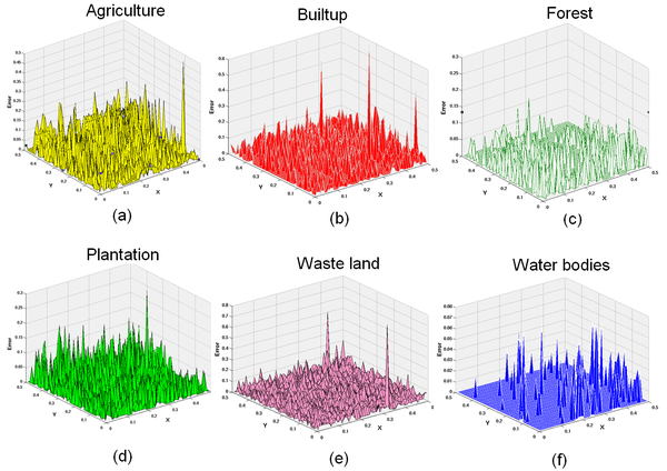
Figure 15. Error distribution of MODIS abundance obtained from HMM (X and Y axes are the two dimensions in feature space and Z axis is the absolute difference between real/reference and estimated class proportion) for the six classes.
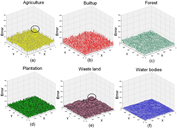
Figure 16. For the HMM, the graph shows the percent of pixels that lie within a given percent of the actual class proportion.
The non-linear model uses abundance vectors and associated true mixture vectors from a training set to estimate mixtures from spectra by interpolation. MLP has several experimental parameters that affect the model’s performance at a certain level such as the number of hidden layers, learning rate, momentum, epoch, etc. We started with a simple architecture with one hidden layer and varied the other parameters.
The algorithm took 7 seconds to train and 7 seconds to generate the fraction images (refer to
Table 1). For MODIS data, the performance of MLP model was stable and acceptable with lowest RMSE in 2000 epochs, 0.7 learning rate, 0.02 momentum and took 18 seconds to train and 9 seconds to generate fraction images (refer Table 3). The correlation is high and significant for both artificial and MODIS data for the HMM compared to the LMM. This implies that training constitutes a vital stage in MLP-based classification. Fifteen percent of the LMM based abundances along with the actual abundances were used for training and the MLP model could interpolate to produce many more combinations of class proportions to match the testing samples.
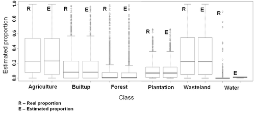
Box plot analysis of the real and estimated proportions for each class indicated that all the classes except water had medians at the same location for both real and estimated proportions. Many pixels both have absence (0%) and full presence (100%) of agriculture. Since the median lies towards the 1st quartile, most of the pixels have less abundance (Figure 17). Many pixels have zero or only a small proportion of built-up and forest with some outliers. Wasteland presents a similar picture as that of agriculture with both absence and full presence, indicating that agriculture and wasteland are the two dominant categories in the area. There is a much smaller number of water bodies and most of them are small in area (≤1000 m2), unevenly distributed as captured by classified image. However, these have not been properly estimated by the algorithm as can also be seen in the box plot. This could be due to the size of water bodies that are smaller than the intrinsic scale of the MODIS pixels, and hence the absence of pure pixel for endmembers, which was not detected by N-FINDR algorithm. The experiments performed in this analysis also indicated areas where non-linear detection methods for targets in hyper spectral imagery have proven to be more effective than linear methods. These scenarios may be targets of small abundance situations, where small target areas are dispersed throughout the image or situations were accuracy is required. Since the approach in this work is a hybrid of linear and non-linear estimators, it can be easily acclimatized to either the linear on
non-linear mixture model.
Figure 17. Box plot of the actual and estimated proportions
Initialization and training are the two issues in a MLP network that have to be dealt with carefully. However, an effective learning algorithm should not depend on initial conditions, which can only affect the convergence rate but should not alter the final results [32]. This is not the case of learning algorithms used for NNs. In order for a mixture model to be effective, initial values must be representative and cannot be arbitrary. In a recent study, Plaza et al. [33] used ANN based models to select higher informative samples in order to effectively train the neural architecture using (1) a border-training algorithm which selects training samples located in the vicinity of the hyperplanes that can optimally separate the classes; (2) a mixed-signature algorithm to select the most spectrally mixed pixels; and (3) a morphological-erosion algorithm which incorporates spatial information through mathematical morphology to select spectrally mixed training samples located in spatially homogeneous regions. The experimental results were demonstrated using non-linear mixed spectra with absolute ground truth.
The non-linear mixture output also depends on selection of endmembers, which is an important issue for successful application of this approach. One of the potential drawbacks of the N-FINDR algorithm is that it requires at least one pixel in the image to be pure. This may not always be the case. In such cases, alternative methods of endmember extraction have to be studied and integrated in the algorithm. Also, the simulated dataset in our work is noise-free (has no noise component) so, further research is required to analyze the impact of the interference of noise.
|
