|
The methods adopted in the analysis involved:
1. Creation of base layers: Base layers like district boundary, district with taluk and village boundaries, road network, drainage network, mapping of water bodies, etc. from the SOI toposheets of scale 1:250000 and 1:50000.
2. Georeferencing of acquired remote sensing data to latitude-longitude coordinate system with Evrst 56 datum: Landsat bands, IRS LISS-III MSS bands, MODIS bands 1 and 2 (spatial resolution 250 m) and bands 3 to 7 (spatial resolution 500 m) were geocorrected with the known ground control points (GCP’s) and projected to Polyconic with Evrst 1956 as the datum, followed by masking and cropping of the study area.
3. Resampling using nearest neighbourhood technique:
- Band 1, 2, 3 and 4 of Landsat 1973 data to 79 m.
- Band 1, 2, 3 and 4 of Landsat TM of 1992 to 30 m.
- Band 1, 2, 3, 4, 5 and 7 of Lansat ETM+ to 30 m.
- MODIS bands 1 to 7 to 250 m.
- IRS LISS-III band 1, 2 and 3 to 23.5 m.
- Thermal band of TM (resampled to 120 m), ETM+ (to 60 m) and MODIS (to 1 km) and Panchromatic bands of ETM+ (resampled to 15 m).
4. Computation of Shannon’s Entropy: The Shannon’s entropy (Yeh and Li, 2001) was computed to detect the urban sprawl phenomenon given by equation 1.
 ….. (Equation 1) ….. (Equation 1)
where, Pi is the Proportion of the variable in the ith zone n the total number of zones. This value ranges from 0 to log n, indicating very compact distribution for values closer to 0. The values closer to log n indicates that the distribution is much dispersed. Larger value of entropy reveals the occurrence of urban sprawl.
5. Principal Component Analysis (PCA): Principal components representing maximum variability of the original datasets were chosen based on eigen values. PCA was carried out to reduce the dimensionality with
- Bands 1, 2, 3 and 4 of Landsat MSS data.
- Band 1, 2, 3 and 4 of Landsat TM.
- Band 2, 3, 4, 5 and 7 of Landsat ETM+.
- Bands 1 to 7 of MODIS data (of 2002 and 2007).
The purpose of this process is to compress all the information contained in an original m– band data set into fewer than m“new bands” or components. The new components are then used in lieu of the original data and may be applied as a preprocessing procedure prior to automated classification process of the data.
Let m be the total number of bands and n be the number of pixels in each band. To every pixel, we associate a m-dimensional feature vector with components corresponding to the gray values of the m bands. The sample mean of the pixels is defined by
 ….. (Equation 2) ….. (Equation 2)
where, μ is the mean of the feature vector, xi is the feature vector of the ith pixel and n is the total number of pixels. The covariance matrix is defined as
 ….. (Equation 3) ….. (Equation 3)
In equation 3, the superscript ‘T’ denotes vector transpose. An unbiased estimate of the sample covariance matrix C is given by
 ….. (Equation 4) ….. (Equation 4)
Next, the eigenvalues and eigenvectors of the matrix C are computed by solving
(C − λi * I) * ei = 0 ….. (Equation 5)
where ei = (a1, a2, ..., am)T is the eigenvector corresponding to the eigenvalues λi and I is the identity matrix. The eigenvalues λi ¸ are determined by solving the characteristic equation
| C − λ * I | = 0 ….. (Equation 6)
A new coordinate system is formed by normalized eigenvectors of the covariance (or correlation) matrix C. The mapping of each feature vector x = (x1, x2, x3......xm) on the ith principal component is given by:
 ….. (Equation 7) ….. (Equation 7)
Chosen Principal Components represents maximum variability of the original datasets.
6. Fusion: Image fusion is a concept of combining multiple images of different spatial and spectral resolution into composite images with better spatial and spectral resolution. The result of image fusion is a new image which is more suitable for human and machine perception or further image processing tasks such as segmentation, feature extraction and object recognition (Pajares, G., et al., 2004). RGB – HIS algorithm was used to fuse
- PC1, PC2 and PC3 of Landsat MSS data (of 1973 with a spatial resolution of 79 m) with PC1 of Landsat TM data (of 1992 with a spatial resolution of 30 m).
- Band 2, 3 and 4 of Landsat ETM+ data (of 2000 with a spatial resolution of 30 m) with Landsat ETM+ band 8 (panchromatic data with spatial resolution 15m)
- PC1, PC2 and PC3 of MODIS data (of 2002 and 2007 with a spatial resolution of 250 m) with PC1 of Landsat ETM+ data (of 2000 with a spatial resolution of 30 m).
Finally, Landsat MSS, TM, ETM+ and MODIS data were all at 30 m spatial resolution. In GB – HIS algorithm (Carper, et al., 1990) the low resolution data are transformed to the IHS (I: intensity, H: hue, S: saturation) color space as equation 8, 9 and 10.
 ….. (Equation 8) ….. (Equation 8)
R, G and B corresponds to PC1, PC2 and PC3 (of Landsat MSS and MODIS) or Band 2, 3 and 4 (of Landsat ETM+)
 ….. (Equation 9) ….. (Equation 9)
 ….. (Equation 10) ….. (Equation 10)
Here V1, V2 are the intermediate variables. I is replaced with high spatial resolution image (like PC1 of Landsat TM for fusing with Landsat MSS; PC1 of ETM+ for fusing with MODIS; and Panchromatic band 8 of Landsat ETM+ to fuse with band 2, 3, and 4 of the same sensor). Then, the fused images of high spatial resolution are obtained by performing an inverse transformation of IHS back to the original RGB as given in equation 11.
 ….. (Equation 11) ….. (Equation 11)
7. Supervised Classification using Bayesian Classifier: In supervised classification, the pixel categorization process is done by specifying the numerical descriptors of the various land cover types present in a scene. It involves three steps –
- Training stage: identifying representative training areas and developing a numerical description of the spectral attributes of each land cover type in the scene, known as training set,
- Classification stage: each pixel in the image data set is categorized into the land cover class it most closely resembles, and
- Output stage: the process consists of a matrix of interpreted land cover category types.
The following section discusses the classification strategies that use the training set descriptions of the category spectral response patterns as interpretation keys by which pixels of unidentified cover types are categorised into their appropriate classes.
Training samples were collected according to the classes given by D1,…, Dc (built up, vegetation, water bodies and others), where the samples in Dj were i.i.d (independent and identically distributed) random variables with probability p(x|ωk) having known parametric form, which could be determined uniquely by the value of a parameter vector Өc. Because of dependence of p(x|ωc) on Өc, p(x|ωc) can be written as p(x|ωc, Өc). We use the information provided by training data to obtain estimates for unknown parameter vectors Ө1, Ө12…, Өc. Assuming that samples in Di give no information about Өc if i ≠ c, i:e., parameters for the different classes are functionally independent. So,
 ….. (Equation 12) ….. (Equation 12)
Let Ө denote the p-component vector Ө = (Ө1, …, Өp)T and let  be the gradient operator, so l(Ө) ≡ ln p(D|Ө) that maximizes the log likelihood is be the gradient operator, so l(Ө) ≡ ln p(D|Ө) that maximizes the log likelihood is  over Ө. over Ө.
Now  ….. (Equation 13) ….. (Equation 13)
and  ….. (Equation 14) ….. (Equation 14)
Thus the maximum likelihood estimates for Ө is obtained from the set of p equations,  . A solution to Ө could represent a global, local maximum or minimum out of which one represents a true maximum which is confirmed by the calculating the second derivatives. . A solution to Ө could represent a global, local maximum or minimum out of which one represents a true maximum which is confirmed by the calculating the second derivatives.
In our case, μk and Σk are unknown, so this constitute the components of the parameter vector Ө. Considering the univariate case, with Ө1 = μ and Ө2 = σ2, the log-likelihood of a single point is
 ….. (Equation 15) ….. (Equation 15)
and its derivative is
 ….. (Equation 16) ….. (Equation 16)
Applying the full log-likelihood and rearranging the terms, the maximum-likelihood estimate for multivariate case on substituting the  and and  is is
 ….. (Equation 17) ….. (Equation 17)
 ….. (Equation 18) ….. (Equation 18)
The sample mean and covariance are taken as the maximum-likelihood estimate for the true mean vector and covariance matrix. The covariance matrices are assumed to be different for each category. So the maximum-likelihood quadratic discriminant analysis classifier is
 ….. (Equation 19) ….. (Equation 19)
where
 ….. (Equation 20) ….. (Equation 20)
 ….. (Equation 21) ….. (Equation 21)
 ….. (Equation 22) ….. (Equation 22)
The values of mean  , covariance , covariance  and prior probability and prior probability  are substituted in the discriminant function as given by equation 19. A pixel is assigned to a particular class for which it has the maximum probability. This provided the supervised classified image from which the c classes are obtained. are substituted in the discriminant function as given by equation 19. A pixel is assigned to a particular class for which it has the maximum probability. This provided the supervised classified image from which the c classes are obtained.
8. Accuracy assessment: Accuracy assessments were done with field knowledge, visual interpretation and also referring Google Earth (http://earth.google.com).
9. Computation of Normalised Difference Vegetation Index (NDVI): Vegetated areas have a relatively high Near-IR (Infrared) reflectance and low visible reflectance. Due to this property of the vegetation, various mathematical combinations of the NIR and the Red band have been found to be sensitive indicators of the presence and condition of green vegetation. NDVI is computed using Equation 23:
 ….. (Equation 23) ….. (Equation 23)
It separates green vegetation from its background soil brightness and retains the ability to minimize topographic effects while producing a measurement scale ranging from –1 to +1 with NDVI < 0 representing no vegetation. NDVI is sensitive to the presence of vegetation, since green vegetation usually decreases the signal in the red due to chlorophyll absorption and increases the signal in the NIR wavelength due to light scattering by leaves.
The potential of computing NDVI has created great interest to study global biosphere dynamics. It is preferred to the simple index for global vegetation monitoring because NDVI helps compensate for changing illumination conditions, surface slope, aspect and other extraneous factors. Numerous investigators have related the NDVI to several vegetation phenomena. These phenomena have ranged from vegetation seasonal dynamics at global and continental scales, to tropical forest clearance, leaf area index measurement, biomass estimation, percentage ground cover determination and FPAR (fraction of absorbed photosynthetically active radiation).
10. Derivation of Land Surface Temperature (LST)
10.1. LST from Landsat TM
The TIR band 6 of Landsat-5 TM was used in order to calculate the surface temperature of the area. The digital number (DN) was first converted into radiance LTM using
LTM = 0.124 + 0.00563 * DN ….. (Equation 24)
The radiance was converted to equivalent blackbody temperature TTMSurface at the satellite using
TTMSurface = K2/(K1 – lnLTM) – 273 ….. (Equation 25)
The coefficients K1 and K2 depend on the range of blackbody temperatures. In the blackbody temperature range 260-300K the default values (Singh, S. M., 1988) for Landsat TM are K1 = 4.127 and K2 = 1274.7.
Brightness temperature is the temperature that a blackbody would obtain in order to produce the same radiance at the same wavelength (λ = 11.5 μm). Therefore, additional correction for spectral emissivity (ε) is required to account for the non-uniform emissivity of the land surface. Spectral emissivity for all objects are very close to 1, yet for more accurate temperature derivation emissivity of each land cover class is considered separately. Emissivity correction is carried out using surface emissivities for the specified land covers (table 2) derived from the methodology described in Snyder, et al., (1998) and Stathopoulou, et al. (2006).
Table 2: Surface emissivity values by land cover type
| Land cover type |
Emissivity |
| Densely urban |
0.946 |
| Mixed urban (Medium Built) |
0.964 |
| Vegetation |
0.985 |
| Water body |
0.990 |
| Others |
0.950 |
The procedure involves combining surface emissivity maps obtained from the Normalized Difference Vegetation Index Thresholds Method (NDVITHM) (Sobrino and Raissouni, 2000) with land cover information. The emmissivity corrected land surface temperature (Ts) were finally computed as follows (Artis and Carnhan, 1982)
 ….. (Equation 26) ….. (Equation 26)
where, λ is the wavelength of emitted radiance for which the peak response and the average of the limiting wavelengths (λ = 11.5 μm) (Markham and Barker, 1985) were used, ρ = h x c/σ (1.438 x 10⁻² mK), σ = Stefan Bolzmann’s constant (5.67 x 10⁻⁸ Wm-2K-4 = 1.38 x 10⁻²³ J/K), h = Planck’s constant (6.626 x 10⁻³⁴ Jsec), c = velocity of light (2.998 x 10⁸ m/sec), and ε is spectral emissivity.
10.2. LST from Landsat ETM+
The TIR image (band 6) was converted to a surface temperature map according to the following procedure (Weng, et al., 2004). The DN of Landsat ETM+ was first converted into spectral radiance LETM using equation 27, and then converted to at-satellite brightness temperature (i.e., black body temperature, TETMSurface), under the assumption of uniform emissivity (ε ≈ 1) using equation 28 (Landsat Project Science Office, 2002):
LETM = 0.0370588 x DN + 3.2 ….. (Equation 27)
TETMSurface = K2/ln (K1/ LETM + 1) ….. (Equation 28)
where, TETMSurface is the effective at-satellite temperature in Kelvin, LETM is spectral radiance in watts/(meters squared x ster x μm); and K1 and K2 are pre-launch calibration constants. For Landsat-7 ETM+, K2 = 1282.71K, K1 = 666.09 mWcm-2sr-1μm-1 were used (http://ltpwww.gsfc.nasa.gov/IAS/handbook/handbook_htmls/chapter11/chapter11.html). The emissivity corrected land surface temperatures Ts were finally computed by equation 26.
11. Linear Spectral Unmixing
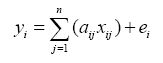
Linear unmixing is used for solving the mixed pixel problem in the case of coarse resolution data. The hypothesis underlying linear unmixing is that the spectral radiance measured by the sensor consists of the radiances reflected by all of these materials, summed in proportion to the sub-pixel area covered by each material. To the degree that, this hypothesis is valid, and that the endmembers (pure pixels or pixels having only one category) are given by the reference spectra of each of the individual pure materials, and under the condition that these spectra are linearly independent, then in theory one can deduce the makeup of the target pixel by calculating the particular combination of the endmember spectra required to synthesize the target pixel spectrum. A brief outline of the method is mentioned below:
Linear spectral unmixing assumes that the spectrum measured by a sensor is a linear combination of the spectra of all components within the pixel. Therefore,
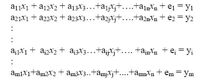
where,
- m = Nmber of bands in the multispectral data set
- n = Number of distinct classes of objects.
- y1, 2, …., m = Spectral reflectance of the pixel in 1st, 2nd, 3rd, …, mth spectral band of a pixel contain one or more components
- aij = Spectral reflectance of the jth component in the pixel for ith spectral band.
- xj = Proportion value of the jth component in the pixel
- ei = Error term for the ith spectral band
- j = 1, 2, 3 ... n (Number of components assumed)
- i = 1, 2, 3 ... m (Number of Spectral bands for the sensor system)
The error term (ei) is due to the assumption made that the response of each pixel in any spectral wavelength is a linear combination of the proportional responses of each component. The above equations can also be written as:
or, AX=Y, assuming that the error term is 0.
Then, AX-Y≈ 0 (if e1, e2, …, ei, …, em = 0)
where, A is a m x n matrix (a11, a12, …, amn), X is a n x 1 vector (x1, x2, …, xn) and Y is a n x 1 vector (y1, y2, …, yn). Therefore, the above set of equations can be written as,
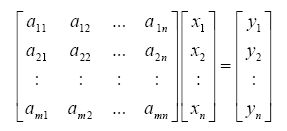
If m < n, many solutions exist; if m = n and A is invertible (full rank matrix), a solution exist and it is unique; if m > n, (a) solution may not exist (b) a unique solution exists. The solution of x is obtained by minimizing the function ||AX – Y||. Various solutions can be obtained when ||AX – Y|| is minimized with different constraints on x.
Unconstrained case:
x1+x2+…+xn ≠ 1, where x is any arbitrary real number. Now our aim is to minimize the difference between AX and Y so that the error term is zero. Since A, X and Y are vectors, so the difference (length) or norm of these vectors can be given by
||AX – Y||2
= (AX – Y)T (AX – Y)
= ((AX)T – YT) (AX – Y)
= ATXTAX – XTATY – YTAX + YTY ….. (Equation 29)
Considering the 3rd term YTAX, let AX=Z, YTAX= YTZ=ZTY.
Therefore, YTAX = (AX) TY= XTATY. Now, equation 29 can be written as
= ATXTAX – XTATY – XTATY + YTY
= ATXTAX + YTY – 2XTATY
Assume J= ATXTAX + YTY – 2XTATY
Differentiating w.r.t X

ATAX = ATY
 ….. (Equation 30) ….. (Equation 30)
which is termed as the Unconstrained Least Squares (ULS) estimate of the abundance. The negative abundance values can be considered to be zero and the values exceeding one can be considered to be 1.
Constrained case:
Imposing the sum-to-one constraint on the abundance values i.e. x1+x2+…+xn = 1 or  . .
The solution to the above problem can be solved by minimizing the function
J(X, λ) = AX – Y + λ (1TX – 1) where λ is the Lanrangian multiplier. The purpose of introducing the Lanrangian multiplier is to convert the constrained case to the unconstrained case for which we have the above solution.
Proceeding as earlier,
||AX – Y||2 + λ (1TX – 1)
= (AX – Y)T (AX – Y) + λ (1TX – 1)
= ((AX)T – YT) (AX – Y) + λ (1TX – 1)
= ATXTAX – XTATY – YTAX + YTY + λ (1TX – 1)
= ATXTAX + YTY – 2XTATY + λ (1TX – 1)
Differentiating J(X, λ) w.r.t. X
 ….. (Equation 31) ….. (Equation 31)
Differentiating J(X, λ) w.r.t. λ
 or, or, 
Now, from equation 9,

or, 
or, 
or,  ….. (Equation 32) ….. (Equation 32)
Multiplying both sides by 1T,
or, 
therefore, 
so,  (since 1TX=1) ….. (Equation 33) (since 1TX=1) ….. (Equation 33)
Equation 33 can also be written as 
Substituting the value of λ from equation (33) in equation (32), we get,

 ….. (Equation 34) ….. (Equation 34)
Equation 34 gives the Constrained Least Squares (CLS) estimate of the abundance.
12. Catchment yield and land use
Flows at the catchment were indirectly estimated by the land use area, runoff coefficient and precipitation. Land use is the use of land by humans, usually with emphasis on the functional role of land such as land under buildings, plantation, pastures, etc. Land use pattern in the catchment has direct implications on hydrological yield. The yield of a catchment area is the net quantity of water available for storage, after all losses, for the purpose of water resource utilization and planning (Ramachandra, et al. 1999). Runoff is the balance of rainwater, which flows or runs over the natural ground surface after losses by evaporation, interception and infiltration. The runoff from rainfall was estimated by rational method that is used to obtain the yield of a catchment area by assuming a suitable runoff coefficient.
Yield = C*A*P ….. (Equation 35)
where, C: runoff coefficient, A: catchment area and P: rainfall.
The value of C varies depending on the soil type, vegetation, geology, etc. from 0.1 to 0.2 (heavy forest), 0.2 to 0.3 (sandy soil), 0.3 to 0.4 (cultivated absorbent soil), 0.4 to 0.6 (cultivated or covered with vegetation), 0.6 to 0.8 (slightly permeable, bare) to 0.8 to 1.0 (rocky and impermeable).
|