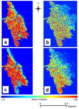
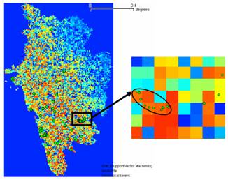
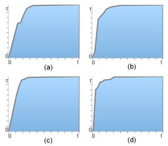
Results and Discussion

Two different precipitation layers were used to predict landslides – precipitation of wettest month and precipitation in the wettest quarter of the year along with the seven other layers as mentioned in section III. Figure 6 (a) and (b) are the landslide probability maps using GARP and SVM on precipitation of wettest month. The landslide occurrence points were overlaid on the probability maps to validate the prediction as shown in Fig. 7. The GARP map had an accuracy of 92% and SVM map was 96% accurate with respect to the ground and Kappa values 0.8733 and 0.9083 respectively. The corresponding ROC curves are shown in Fig. 8 (a) and (b). Total area under curve (AUC) for Fig. 8 (a) is 0.87 and for Fig. 8 (b) is 0.93. Figure 6 (c) and (d) are the landslide probability maps using GARP and SVM on precipitation of wettest quarter with accuracy of 91% and 94% and Kappa values of 0.9014 and 0.9387 respectively.

Fig. 6. Probability distribution of the landslide prone areas.

ROC curves in figure 8 (c) and (d) show AUC as 0.90 and 0.94. Various measures of accuracy were used as per [46] to assess the outputs. Table I presents the confusion matrix structure indicating true positives, false positives, false negatives and true negatives.

Fig. 7. Validation of the probability distribution of the landslide prone areas by overlaying landslide occurrence points.

Confusion matrices were generated for each of the 4 outputs (Table II) and different measures of accuracy such as prevalence, global diagnostic power, correct classification rate, sensitivity, specificity, omission and commission error were computed as listed in Table III.

Fig. 8. ROC curves for landslide prone maps (a) GARP (b) SVM on precipitation of wettest month; (c) GARP and (d) SVM on precipitation of wettest quarter.

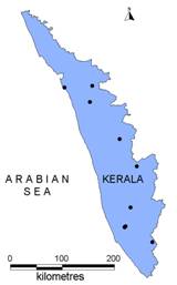
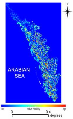
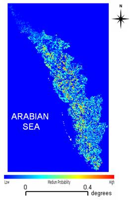
The results indicate that the output obtained from SVM using precipitation of the wettest month was best among the 4 scenarios. It maybe noted that the outputs from GARP for both the wettest precipitation month and quarter are close to the SVM in term of accuracy. One reason is that, most of the areas have been predicted as probable landslide prone zones (indicated in red in Fig. 6 (a) and (c)) and the terrain is highly undulating with steep slopes that are frequently exposed to landslides induced by rainfall. Obviously, the maximum number of landslide points occurring in the undulating terrain, collected from the ground will fall in those areas indicating that they are more susceptible to landslides compared to north-eastern part of the district which has relatively flat terrain.

Another case study of Kerala state, India was carried out with the same environmental layers along with 10 landslide occurrence points as shown in Fig. 9. The predicted output for precipitation in the wettest month is shown in Fig. 10 and precipitation in the wettest quarter is shown in Fig. 11 with an overall accuracy of 60%. The Kappa values for two cases were 0.966335 and 0.96532. The ROC curves are shown in Fig. 12 (a) and (b) with 0.97 AUC for both the cases respectively. The confusion matrix and statistics are presented in Table IV and V. The reason for low accuracy is the presence of only 10 occurrence points throughout the state. Also, the coarse resolution of the pixel may be attributed for poor accuracy. However, the Kappa value and the AUC are high which indicate that the probability distribution of the predicted points fall well within the occurrence points. It is another matter that the intensity of these landslide points may vary from low to medium to high. One potential limitation of the above data is their spatial resolution – 1 km. It is highly unlikely that landslides of this magnitude can occur in the study area. However, given the environmental layers along with the occurrence points, the probable areas of occurrence can be mapped with great certainty.

The movement of a slope is complex and it is induced or perturbed by many other factors besides rainfall such as groundwater data, soil moisture information, etc. which were not used in the prediction. It is known that there are accelerations of slope movements after intense rainfall, however, to what extent rainfall affects the slope movement remains unknown and the correlation between rainfall and the slope movement could be ambiguous in absence of detailed observations. Timely rainfall, soil moisture, grain-size, lithology, geological structure, seismological observations and the longer time intervals for which data are available can improve the accuracy of the model. Beyond their key role in identifying and mapping the landslides, the choice of the variables (environmental layers) used for the prediction are also closely involved. Some limitations of the data set cannot be overcome. In this study for example, no hydrological field data were available. However, significant results were obtained in the study because the variables most influential on landslide were used.

Natural disasters have drastically increased over the last decades. National, state and local government including NGOs are concerned with the loss of human life and damage to property caused by natural disasters. The trend of increasing incidences of landslides occurrence is expected to continue in the next decades due to urbanisation, continued anthropogenic activities, deforestation in the name of development and increased regional precipitation in landslide-prone areas due to changing climatic patterns [47]. The application of modern technologies required to control the effects of natural hazards including landslides must consider three significant factors - prediction, monitoring and conservation. In fact, the promotion of accessibility to urban facilities, such as homes and new roads in mountainous areas is difficult to achieve without considering geological and geotechnical factors to ensure that the development is pleasant and safe. Therefore, it is desired to have a notion about the main factors controlling the slope instability, assessing its severity, discriminating areas with presence/absence of landslides, updating and interpreting landslide data and determining areas that are prone to landslides. In this regard, the present work may be a contribution to the beginning of such disaster and mitigation studies.

Fig. 9. Landslide occurrence points in Kerala.

Fig. 10. Probability distribution of the landslide prone areas in Kerala using precipitation in the wettest month data.

Fig. 11. Probability distribution of the landslide prone areas in Kerala using precipitation in the wettest quarter data.

Fig. 12. ROC curves for the predicted landslide prone maps of Kerala.
(a) using precipitation of the wettest month, (b) using precipitation of the wettest quarter.