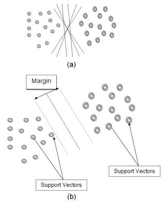
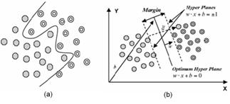
Methods

A. Genetic Algorithm for Rule-set Prediction (GARP): GARP is based on genetic algorithms originally meant to generate niche models for biological species. In this case, the models describe environmental conditions under which the species should be able to maintain populations. GARP is used in the current work here to predict the locations susceptible for landslides with the known landslide occurrence points.

For input, GARP uses a set of point localities where the landslide is known to occur and a set of geographic layers representing the environmental parameters that might limit the landslide existence. Genetic Algorithms (GAs) are a class of computational models that mimic the natural evolution to solve problems in a wide variety of domains. GAs are suitable for solving complex optimisation problems and for applications that require adaptive problem-solving strategies. They are also used as search algorithms based on mechanics of natural genetics that operates on a set of individual elements (the population) and a set of biologically inspired operators which can change these individuals. It maps strings of numbers to each potential solution and then each string becomes a representation of an individual. Then the most promising in its search is manipulated for improved solution [33]. The model developed by GARP is composed of a set of rules. These set of rules is developed through evolutionary refinement, testing and selecting rules on random subsets of training data sets. Application of a rule set is more complicated as the prediction system must choose which rule of a number of applicable rules to apply. GARP maximises the significance and predictive accuracy of rules without overfitting. Significance is established through a χ² test on the difference in the probability of the predicted value before and after application of the rule. GARP uses envelope rules, GARP rules, atomic and logit rules. In envelope rule, the conjunction of ranges for all of the variables is a climatic envelope or profile, indicating geographical regions where the climate is suitable for that entity, enclosing values for each parameter. A GARP rule is similar to an envelope rule, except that variables can be irrelevant. An irrelevant variable is one where points may fall within the whole range. An atomic rule is a conjunction of categories or single values of some variables. Logit rules are an adaptation of logistic regression models to rules. A logistic regression is a form of regression equation where the output is transformed into a probability [34].

B. Support Vector Machine (SVM): SVM are supervised learning algorithms based on statistical learning theory, which are considered to be heuristic algorithms [35]. SVM map input vectors to a higher dimensional space where a maximal separating hyper plane is constructed. Two parallel hyper planes are constructed on each side of the hyper plane that separates the data. The separating hyper plane maximises the distance between the two parallel hyper planes. An assumption is made that the larger the margin or distance between these parallel hyper planes, the better the generalisation error of the classifier will be. The model produced by support vector classification only depends on a subset of the training data, because the cost function for building the model does not take into account training points that lie beyond the margin [35].

In order to classify n-dimensional data sets, n-1 dimensional hyper plane is produced with SVMs. As it seen from Fig. 1 [35], there are various hyper planes separating two classes of data. However, there is only one hyper plane that provides maximum margin between the two classes [35] (Fig. 2), which is the optimum hyper plane. The points that constrain the width of the margin are the support vectors.

In the binary case, SVMs locates a hyper plane that maximises the distance from the members of each class to the optimal hyper plane. If there is a training data set containing m number of samples represented by {x_i, y_i}      (i =1, ... , m), where x ε RN, is an N-dimensional space, and    y ε {-1, +1} is class label, then the optimum hyper plane maximises the margin between the classes. As in Fig. 3, the hyper plane is defined as (w.x_i + b = 0) [35], where x is a point lying on the hyper plane, parameter w determines the orientation of the hyper plane in space, b is the bias that the distance of hyper plane from the origin. For the linearly separable case, a separating hyper plane can be defined for two classes as:

w . x_i + b ≥ +1 for all y = +1                             (1)
w . x_i + b ≤  -1 for all y = -1                             (2)

These inequalities can be combined into a single inequality:
y_i (w. x_i + b ) – 1 ≥ 0                                        (3)
The training data points on these two hyper planes, which are parallel to the optimum hyper plane and defined by the functions w. x_i+ b = ±1, are the support vectors [36]. If a hyper plane exists that satisfies (3), the classes are linearly separable. Therefore, the margin between these planes is equal to 2/||w|| [37]. As the distance to the closest point is 2/||w||, the optimum separating hyper plane can be found by minimizing ||w||² under the constraint (3).

Fig. 1. (a) Hyper planes for linearly separable data, (b) Optimum hyper plane and support vectors [35].

Fig. 2. Support vectors and optimum hyper plane for the binary case of linearly separable data sets [35].

Thus, determination of optimum hyper plane is required to solve optimisation problem given by:

min(0.5*||w||² )                                   (4)

subject to constraints,

y_i (w. x_i + b ) ≥ -1   and y_i  ε {+1, -1}                         (5)

As illustrated in Fig. 3 (a) [35], nonlinearly separable data is the case in various classification problems as in the classification of remotely sensed images using pixel samples. In such cases, data sets cannot be classified into two classes with a linear function in input space. Where it is not possible to have a hyper plane defined by linear equations on the training data, the technique can be extended to allow for nonlinear decision surfaces [38, 39].

Fig. 3. (a) Separation of nonlinear data sets, (b) Generalisation of the solution by introducing slack variable for nonlinear data [35].

Thus, the optimisation problem is replaced by introducing  slack variable (Fig. 3(b)).

                                            (6)

subject to constraints,

                          (7)

where C is a regularisation constant or penalty parameter. This parameter allows striking a balance between the two competing criteria of margin maximisation and error minimisation, whereas the slack variables  indicates the distance of the incorrectly classified points from the optimal hyper plane [40]. The larger the C value, the higher the penalty associated to misclassified samples [41].

When it is not possible to define the hyper plane by linear equations, the data can be mapped into a higher dimensional space (H) through some nonlinear mapping functions (Ф). An input data point x is represented as Ф(x) in the high-dimensional space. The expensive computation of (Ф(x).Ф(x_i)) is reduced by using a kernel function [36]. Thus, the classification decision function becomes:

                                (8)

where for each of r training cases there is a vector (xi) that represents the spectral response of the case together with a definition of class membership (y_i).α_i (i = 1,….., r) are Lagrange multipliers and K(x, x_i) is the kernel function. The magnitude of α_i is determined by the parameter C [42]. The kernel function enables the data points to spread in such a way that a linear hyper plane can be fitted [43]. Kernel functions commonly used in SVMs can be generally aggregated into four groups; namely, linear, polynomial, radial basis function and sigmoid kernels. The performance of SVMs varies depending on the choice of the kernel function and its parameters.  A free and open source software – openModeller [44] was used for predicting the probable landslide areas. openModeller (http://openmodeller.sourceforge.net/) is a flexible, user friendly, cross-platform environment where the entire process of conducting a fundamental niche modeling experiment can be carried out. It includes facilities for reading landslide occurrence and environmental data, selection of environmental layers on which the model should be based, creating a fundamental niche model and projecting the model into an environmental scenario using a number of algorithms as shown in Fig. 4.

Fig. 4. Methodology used for landslide prediction in openModeller.