Insights to Urban Dynamics through Landscape Spatial Pattern Analysis

Urbanisation is a dynamic complex phenomenon involving large scale changes in the land uses at local levels. Analyses of changes in land uses in urban environments provide a historical perspective of land use and give an opportunity to assess the spatial patterns, correlation, trends, rate and impacts of the change, which would help in better regional planning and good governance of the region. Main objective of this research is to quantify the urban dynamics using temporal remote sensing data with the help of well-established landscape metrics. Bangalore being one of the rapidly urbanizing landscapes in India has been chosen for this investigation. Complex process of urban sprawl was modelled using spatio temporal analysis. Land use analyses show 584% growth in built-up area during the last four decades with the decline of vegetation by 66% and water bodies by 74%. Analyses of the temporal data reveals an increase in urban built up area of 342.83% (during 1973 to 1992), 129.56% (during 1992 to 1999), 106.7% (1999 to 2002), 114.51% (2002 to 2006) and 126.19% from 2006 to 2010. The Study area was divided into four zones and each zone is further divided into 17 concentric circles of 1 km incrementing radius to understand the patterns and extent of the urbansiation at local levels. The urban density gradient illustrates radial pattern of urbanization for the period 1973 to 2010. Bangalore grew radially from 1973 to 2010 indicating that the urbanization is intensifying from the central core and has reached the periphery of the Greater Bangalore. Shannon’s entropy, alpha and beta population densities were computed to understand the level of urbanization at local levels. Shannon's entropy values of recent time confirms dispersed haphazard urban growth in the city, particularly in the outskirts of the city. This also illustrates the extent of influence of drivers of urbanization in various directions. Landscape metrics provided in depth knowledge about the sprawl. Principal component analysis helped in prioritizing the metrics for detailed analyses. The results clearly indicates that whole landscape is aggregating to a large patch in 2010 as compared to earlier years which was dominated by several small patches. The large scale conversion of small patches to large single patch can be seen from 2006 to 2010. In the year 2010 patches are maximally aggregated indicating that the city is becoming more compact and more urbanised in recent years. Bangalore was the most sought after destination for its climatic condition and the availability of various facilities (land availability, economy, political factors)compared to other cities. The growth into a single urban patch can be attributed to rapid urbanisation coupled with the industrialisation. Monitoring of growth through landscape metrics helps to maintain and manage the natural resources.

Keywords: Urbanisation, urban sprawl, landscape metrics, spatial metrics, remote sensing

I. Introduction

Urbanization and Urban Sprawl: Urbanisation is a dynamic process involving changes in vast expanse of land cover with the progressive concentration of human population. The process entails switch from spread out pattern of human settlements to compact growth in urban centres. Rapidly urbanising landscapes attains inordinately large population size leading to gradual collapse in the urban services evident from the basic problems in housing, slum, lack of treated water supply, inadequate infrastructure, higher pollution levels, poor quality of life, etc. Urbanisation is a product of demographic explosion and poverty induced rural-urban migration. Globalisation, liberalization, privatization are the agents fuelling urbanization in most parts of India. However, unplanned urbanization coupled with the lack of holistic approaches, is leading to lack of infrastructure and basic amenities. Hence proper urban planning with operational, developmental and restorative strategies is required to ensure the sustainable management of natural resources.

Urban dynamics involving large scale changes in the land use depend on (i) nature of land use and (ii) the level of spatial accumulation. Nature of land use depends on the activities that are taking place in the region while the level of spatial accumulation depends on the intensity and concentration. Central areas have a high level of spatial accumulation of urban land use (as in the CBD: Central Business District), while peripheral areas have lower levels of accumulation. Most economic, social or cultural activities imply a multitude of functions, such as production, consumption and distribution. These functions take place at specific locations depending on the nature of activities – industries, institutions, etc.

Unplanned growth would involve radical land use conversion of forests, surface water bodies, etc. with the irretrievable loss of ground prospects (Pathan et al., 1989, 1991, 1993, 2004). The process of urbanization could be either in the form of townships or unplanned or organic. Many organic towns in India are now influencing large scale infrastructure development, etc. due to the impetus from the National government through development schemes such as JNNURM (Jawaharlal Nehru National Urban Renewal Mission), etc. The focus is on the fast track development through an efficient infrastructure and delivery mechanisms, community participation, etc.

The urban population in India is growing at about 2.3% per annum with the global urban population increasing from 13% (220 million in 1900) to 49% (3.2 billion, in 2005) and is projected to escalate to 60% (4.9 billion) by 2030 (Ramachandra and Kumar, 2008; World Urbanization Prospects, 2005). The increase in urban population in response to the growth in urban areas is mainly due to migration. 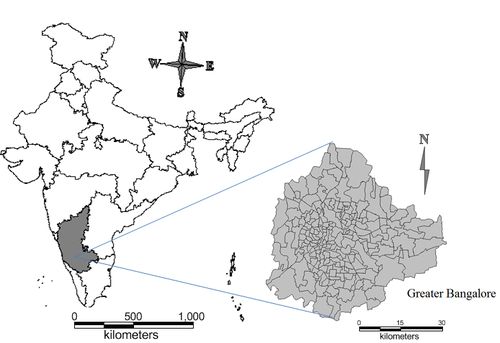There are 48 urban agglomerations/cities having a population of more than one million in India (in 2011).

Urbanisation often leads to the dispersed haphazard development in the outskirts, which is often referred as sprawl. Thus urban sprawl is a consequence of social and economic development of a certain region under certain circumstances. This phenomenon is also defined as an uncontrolled, scattered suburban development that depletes local resources due to large scale land use changes involving the conversion of open spaces (water bodies, parks, etc.) while increasing carbon footprint through the spurt in anthropogenic activities and congestion in the city (Peiser, 2001, Ramachandra and Kumar, 2009). Urban sprawl increasingly has become a major issue facing many metropolitan areas. Due to lack of visualization of sprawl a priori, these regions are devoid of any infrastructure and basic amenities (like supply of treated water, electricity, sanitation facilities). Also these regions are normally left out in all government surveys (even in national population census), as this cannot be grouped under either urban or rural area. Understanding this kind of growth is very crucial in order to provide basic amenities and more importantly the sustainable management of local natural resources through decentralized regional planning.

Urban sprawl has been captured indirectly through socioeconomic indicators such as population growth, employment opportunity, number of commercial establishments, etc. (Brueckner, 2000; Lucy and Phillips, 2001). However, these techniques cannot effectively identify the impacts of urban sprawl in a spatial context. In this context, availability of spatial data at regular interval through space-borne remote sensors are helpful in effectively detecting and monitoring rapid land use changes (e.g., Chen, et al., 2000; Epstein, et al., 2002; Ji et al., 2001; Lo and Yang, 2002; Dietzel et al., 2005). Urban sprawl is characterised based on various indicators such as growth, social, aesthetic, decentralisation, accessibility, density, open space, dynamics, costs, benefits, etc. (Bhatta et al., 2009a, 2009b, 2010). Further, Galster et al. (2001), has identified parameters such as density, continuity, concentration, clustering, centrality, nuclearity, proximity and mixed uses for quantifying sprawl. Urbanisation and sprawl analysis would help the regional planners and decision makers to visualize growth patterns and plan to facilitate various infrastructure facilities. In the context of rapid urban growth, development should be planned and properly monitored to maintain internal equilibrium through sustainable management of natural resources. Internal equilibrium refers to the urban system and its dynamics evolving harmony and thus internally limiting impacts on the natural environment consequent to various economic activities with the enhanced growth of population, infra-structure, services, pollution, waste, etc. (Barredo and Demicheli, 2003). Due to globalisation process, the cities and towns in India are experiencing rapid urbanization consequently lacking appropriate infrastructure and basic amenities. Thus understanding the urban dynamics considering social and economic changes is a major challenge. The social and economic dynamics trigger the change processes in urban places of different sizes ranging from large metropolises, cities and small towns. In this context, the analysis of urban dynamics entails capturing and analyzing the process of changes spatially and temporally (Sudhira et al., 2004; Tian, et al., 2005; Yu and Ng, 2007).

Land use Analysis and Gradient approach: The basic information about the current and historical land cover and land use plays a major role in urban planning and management (Zhang et al., 2002). Land-cover essentially indicates the feature present on the land surface (Janssen, 2000; Lillesand and Keifer, 2002; Sudhira et al., 2004). Land use relates to human activity/economic activity on piece of land under consideration (Janssen, 2000; Lillesand and Keifer, 2002; Sudhira et al., 2004). This analysis provides various uses of land as urban, agriculture, forest, plantation, etc., specified as per USGS classification system (http://landcover.usgs.gov/pdf/anderson.pdf) and National Remote Sensing Centre, India (http://www.nrsc.gov.in). Mapping landscapes on temporal scale provide an opportunity to monitor the changes, which is important for natural resource management and sustainable planning activities. In this regard, “Density Gradient metrics” with the time series spatial data analysis are potentially useful in measuring urbanisation and sprawl (Torrens and Alberti, 2000). Density gradient metrics include sprawl density gradient, Shannon’s entropy, alpha and beta population densities, etc. This paper presents temporal land use analysis for rapidly urbanizing Bangalore and density gradient metrics have been computed to evaluate and monitor urban dynamics. Landscape dynamics have been unraveled from temporally discrete data (remote sensing data) through spatial metrics (Crews-Meyer, 2002). Landscape metrics (longitudinal data) integrated with the conventional change detection techniques would help in monitoring land use changes (Rainis, 2003; Narumalani et al., 2004). This has been demonstrated through the application in many regions (Kienast, 1993; Luque et al., 1994; Simpson et al., 1994; Thibault and Zipperer, 1994; Hulshoff, 1995; Medley et al., 1995; Zheng et al., 1997; Palang et al., 1998; Sachs et al., 1998; Pan et al., 1999; Lausch and Herzog, 1999).

Further, landscape metrics were computed to quantify the patterns of urban dynamics, which helps in quantifying spatial patterns of various land cover features in the region (McGarigal and Marks, 1995) and has been used effectively to capture urban dynamics similar to the applications in landscape ecology (Gustafson, 1998; Turner et al., 2001) for describing ecological relationships such as connectivity and adjacency of habitat reservoirs (Geri et al., 2009; Jim and Chen, 2009). Herold et al. (2002, 2003) quantifies urban land use dynamics using remote sensing data and landscape metrics in conjunction with the spatial modelling of urban growth. Angel et al. (2007) have considered five metrics for measuring the sprawl and five attributes for characterizing the type sprawl. Spatial metrics were used for effective characterisation of the sprawl by quantifying landscape attributes (shape, complexity, etc.). Jiang et al. (2007) used 13 geospatial indices for measuring the sprawl in Beijing and proposed an urban sprawl index combining all indices. This approach reduces computation and interpretation time and effort. However, this approach requires extensive data such as population, GDP, land-use maps, floor-area ratio, maps of roadways/highways, urban city centre spatial maps, etc. This confirms that landscape metrics aid as important mathematical tool for characterising urban sprawl efficiently. Population data along with geospatial indices help to characterise the sprawl (Ji et al., 2006) as population is one of the causal factor driving land use changes. These studies confirm that spatio-temporal data along with landscape metrics, population metrics and urban modelling would help in understanding and evaluating the spatio temporal patterns of urban dynamics.

II. Objective:

The objective of this study is to understand the urbanization and urban sprawl process in a rapidly urbanizing landscape, through spatial techniques involving temporal remote sensing data, geographic information system with spatial metrics. This involved (i) temporal analysis of land use pattern, (ii) exploring interconnection and effectiveness of population indices, Shannon's entropy for quantifying and understanding urbanisation and (iii) understanding the spatial patterns of urbanization at landscape level through metrics.

III. Study area:

The study has been carried out for a rapidly urbanizing region in India. Greater Bangalore is the administrative cultural, commercial, industrial, and knowledge capital of the state of Karnataka, India with an area of 741 sq. km. and lies between the latitudes 12°39’00’’ to 13°13’00’’ N and longitude 77°22’00’’ to 77°52’00’’ E. Bangalore city administrative jurisdiction was redefined in the year 2006 by merging the existing area of Bangalore city spatial limits with 8 neighboring Urban Local Bodies (ULBs) and 111 Villages of Bangalore Urban District. Bangalore has grown spatially more than ten times since 1949 (~69 square kilometers to 716 square kilometers) and is the fifth largest metropolis in India currently with a population of about 7 million (Ramachandra and Kumar, 2008). Bangalore city population also has increased enormously from 65,37,124 in 2001 to 95,88,910 in 2011, Which accounts to 46.68 percentage growth in a decade and density of population which was 10732 persons per sq km in 2001 has grown to 13392 persons per sq km.It has a per capita GDP of $2066, which is considerably low with limited expansion to balance both environmental and economic needs.

Figure 1. Study area : Greater Bangalore

IV. Materials & Methods

Urban dynamics was analysed using temporal remote sensing data of the period 1973 to 2010. The time series spatial data acquired from Landsat Series Multispectral sensor (57.5m) and Thematic mapper (28.5m) sensors for the period 1973 to 2010 were downloaded from public domain (http://glcf.umiacs.umd.edu/data). Survey of India (SOI) topo-sheets of 1:50000 and 1:250000 scales were used to generate base layers of city boundary, etc. City map with ward boundaries were digitized from the BBMP (Bruhat Bangalore Mahanagara Palike) map. Population data was collected from the Directorate of Census Operations, Bangalore region (http://censuskarnataka.gov.in). Table1 lists the data used in the current analysis. Ground control points to register and geo-correct remote sensing data were collected using handheld pre-calibrated GPS (Global Positioning System), Survey of India Toposheet and Google earth (http://earth.google.com, http://bhuvan.nrsc.gov.in).

Table 1:  Materials used in the analysis

DATA	Year	Purpose
Landsat Series Multispectral sensor (57.5m)	1973	Land use analysis
Landsat Series Thematic mapper (28.5m) and Enhanced Thematic Mapper sensors	1992,1999, 2002, 2006,2010	Land use analysis
Survey of India (SOI) toposheets of 1:50000 and 1:250000 scales		boundary and base layers.
Census Data	2001	Population density ward-wise

Data analysis

Pre-processing: The remote sensing data obtained were geo-referenced, rectified and cropped pertaining to the study area. Geo-registration of remote sensing data (Landsat data) has been done using ground control points collected from the field using pre calibrated GPS (Global Positioning System) and also from known points (such as road intersections, etc.) collected from geo-referenced topographic maps published by the Survey of India. The Landsat satellite 1973 images have a spatial resolution of 57.5 m x 57.5 m (nominal resolution) were resampled to 28.5m comparable to the 1989 - 2010 data which are 28.5 m x 28.5 m (nominal resolution). 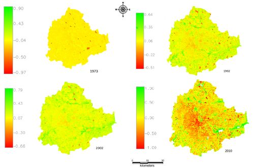Landsat ETM+ bands of 2010 were corrected for the SLC-off by using image enhancement techniques, followed by nearest-neighbour interpolation.

Vegetation Cover Analysis: Normalised Difference Vegetation index (NDVI) was computed to understand the changes in the vegetation cover during the study period. NDVI is the most common measurement used for measuring vegetation cover. It ranges from values -1 to +1. Very low values of NDVI (-0.1 and below) correspond to soil or barren areas of rock, sand, or urban builtup. Zero indicates the water cover. Moderate values represent low density vegetation (0.1 to 0.3), while high values indicate thick canopy vegetation (0.6 to 0.8).

Land use analysis: The method involves i) generation of False Colour Composite (FCC) of remote sensing data (bands – green, red and NIR). This helped in locating heterogeneous patches in the landscape ii) selection of training polygons (these correspond to heterogeneous patches in FCC) covering 15% of the study area and uniformly distributed over the entire study area, iii) loading these training polygons co-ordinates into pre-calibrated GPS, vi) collection of the corresponding attribute data (land use types) for these polygons from the field . GPS helped in locating respective training polygons in the field, iv) supplementing this information with Google Earth v) 60% of the training data has been used for classification, while the balance is used for validation or accuracy assessment.

Land use analysis was carried out using supervised pattern classifier - Gaussian maximum likelihood algorithm. This has been proved superior classifier as it uses various classification decisions using probability and cost functions (Duda et al., 2000). Mean and covariance matrix are computed using estimate of maximum likelihood estimator. Accuracy assessment to evaluate the performance of classifiers (Mitrakis et al., 2008; Ngigi et al., 2008; Gao and Liu, 2008), was done with the help of field data by testing the statistical significance of a difference, computation of kappa coefficients (Congalton et al., 1983; Sha et al., 2008) and proportion of correctly allocated cases (Gao & Liu, 2008). Recent remote sensing data (2010) was classified using the collected training samples. Statistical assessment of classifier performance based on the performance of spectral classification considering reference pixels is done which include computation of kappa (κ) statistics and overall (producer's and user's) accuracies. 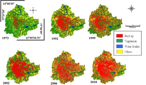For earlier time data, training polygon along with attribute details were compiled from the historical published topographic maps, vegetation maps, revenue maps, etc.

Application of maximum likelihood classification method resulted in accuracy of 76% in all the datasets. Land use was computed using the temporal data through open source program GRASS - Geographic Resource Analysis Support System (http://grass.fbk.eu/). Land use categories include i) area under vegetation (parks, botanical gardens, grass lands such as golf field.), ii) built up (buildings, roads or any paved surface, iii) water bodies (lakes/tanks, sewage treatment tanks), iv) others (open area such as play grounds, quarry regions, etc.).

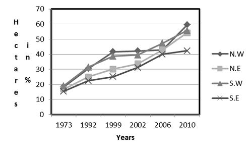
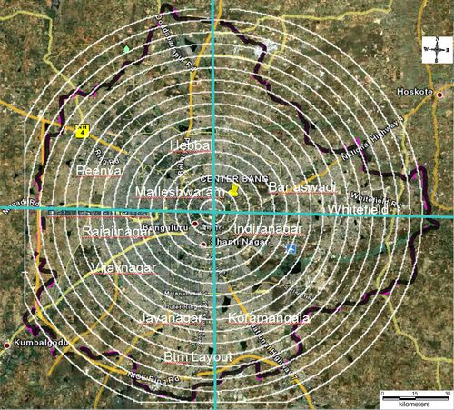
Density Gradient Analysis: Urbanisation pattern has not been uniform in all directions. To understand the pattern of growth vis a vis agents, the region has been divided into 4 zones based on directions - Northwest (NW), Northeast (NE), Southwest (SW) and Southeast (SE) respectively (Figure 2) based on the Central pixel (Central Business district). 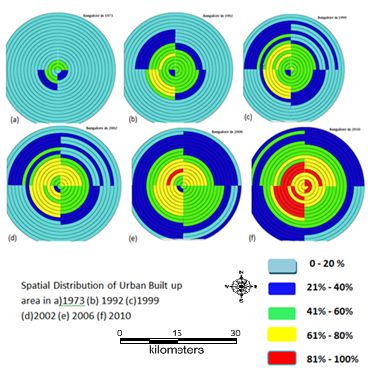The growth of the urban areas in respective zones was monitored through the computation of urban density for different periods.

Division of these zones to concentric circles and computation of metrics: Further each zone was divided into concentric circle of incrementing radius of 1 km radius from the centre of the city (Figure 2), that would help in visualizing and understanding the agents responsible for changes at local level. These regions are comparable to the administrative wards ranging from 67 to 1935 hectares. This helps in identifying the causal factors and locations experiencing various levels (sprawl, compact growth, etc.) of urbanization in response to the economic, social and political forces. This approach (zones, concentric circles) also helps in visualizing the forms of urban sprawl (low density, ribbon, leaf-frog development). The built up density in each circle is monitored overtime using time series analysis.

Figure 2: Division of the study area into concentric circles of incrementing radius of 1km. (Source: Google earth)

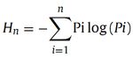
Computation of Shannon’s Entropy: To determine whether the growth of urban areas was compact or divergent the Shannon’s entropy (Yeh and Liu, 2001; Li and Yeh, 2004; Lata et al., 2001; Sudhira et al., 2004; Pathan et al., 2004) was computed for each zones. Shannon's entropy (Hn) given in equation 1, provides the degree of spatial concentration or dispersion of geographical variables among ‘n’ concentric circles across Zones.

                            (1)

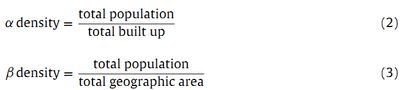
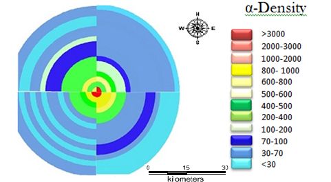
Where Pi is the proportion of the built-up in the i^th concentric circle. As per Shannon’s Entropy, if the distribution is maximally concentrated in one circle the lowest value zero will be obtained. Conversely, if it is an even distribution among the concentric circles will be given maximum of log n.

Computation of Alpha and Beta population density: Alpha and Beta population densities were calculated for each circle with respect to zones. Alpha population density is the ratio of total population in a region to the total builtup area, while Beta population density is the ratio of total population to the total geographical area. These metrics have been often used as the indicators of urbanization and urban sprawl and are given by:

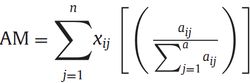
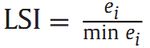
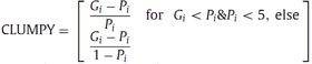
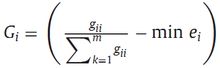
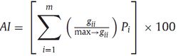
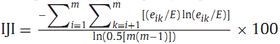
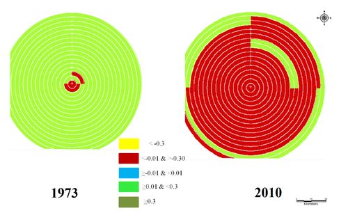
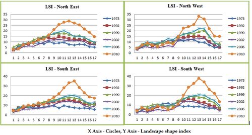
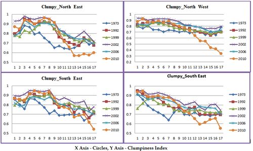
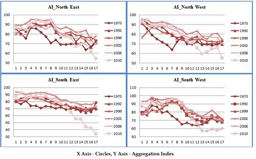
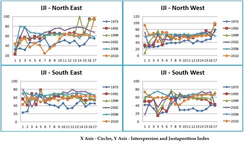
Gradient Analysis of NDVI images of 1973 and 2010: The NDVI gradient was generated to visualize the vegetation cover changes in the specific pockets of the study area.

Calculation of Landscape Metrics: Landscape metrics provide quantitative description of the composition and configuration of urban landscape. 21 spatial metrics chosen based on complexity, centrality and density criteria (Huang et al., 2007) to characterize urban dynamics, were computed zone-wise for each circle using classified land use data at the landscape level with the help of FRAGSTATS (McGarigal and Marks, 1995). The metrics include the patch area (Built up (Total Land Area), Percentage of Landscape (PLAND), Largest Patch Index (Percentage of landscape), Number of Urban Patches, Patch density, Perimeter-Area Fractal Dimension (PAFRAC), Landscape Division Index (DIVISION)), edge/border (Edge density, Area weighted mean patch fractal dimension (AWMPFD), Perimeter Area Weighted Mean Ratio (PARA_AM), Mean Patch Fractal Dimension (MPFD), Total Edge (TE), shape (NLSI(Normalized Landscape Shape Index), Landscape Shape Index (LSI), ), epoch/contagion/ dispersion (Clumpiness, Percentage of Like Adjacencies (PLADJ), Total Core Area(TCA), ENND coefficient of variation, Aggregation index, Interspersion and Juxtaposition). These metrics were computed for each region and Principal Component Analysis was done to prioritise metrics for further detailed analysis. The metrics include the patch area, edge/border, shape, cpoact/contagion/ dispersion and are listed in Appendix I.

Principal Component Analysis: Principal component analysis (PCA) is a multivariate statistical analysis that aids in identifying the patterns of the data while reducing multiple dimensions. PCA through Eigen analysis transforms a number of (possibly) correlated variables into a (smaller) number of uncorrelated variables called principal components. The first principal component accounts for as much of the variability in the data as possible, and each succeeding component accounts for as much of the remaining variability as possible (Wang. 2009). PCA helped in prioritizing eight landscape metrics based on the relative contributions of each metrics in the principal components with maximum variability (Table 2). PCA were performed on the 21 landscape metrics, which helped in prioritizing Landscape metrics. This is done based on the relative contributions of each metrics in the principal components with maximum variability. The new components does represent the original datasets of 21 metrics Based on this, eight landscape metrics were selected for further detailed analysis.

Table 2. Prioritised landscape metrics

	Indicators	Type of metrics and Formula	Range	Significance/ Description
1	Number of Urban Patches	Patch Metrics NP equals the number of patches in the landscape.	NPU>0, without limit.	Higher the value more the fragmentation
2	Perimeter Area Weighted Mean Ratio. PARA_AM	Edge metrics PARA _AM= Pij/Aij Pij = perimeter of patch ij Aij= area weighted mean of patch ij	≥0, without limit	PARA AM is a measure of the amount of 'edge' for a landscape or class. PARA AM value increases with increasing patch shape complexity.
3	Landscape Shape Index (LSI)	Shape Metrics ei =     total length of edge (or perimeter) of class i in terms of number of cell surfaces; includes all landscape boundary and background edge segments involving class i. min ei =   minimum total length of edge (or perimeter) of class i in terms of number of cell surfaces (see below).	LSI>1, Without Limit	LSI = 1 when the landscape is a single square or maximally compact patch; LSI increases without limit as the patch type becomes more disaggregated
4.	Clumpiness	Compactness/ contagion / dispersion metrics gii =number of like adjacencies (joins) between pixels of patch type (class) I based on the double-count method. gik =number of adjacencies (joins) between pixels of patch types (classes) i and k based on the double-count method. min-ei =minimum perimeter (in number of cell surfaces) of patch type (class)i for a maximally clumped class. Pi =proportion of the landscape occupied by patch type (class) i.	-1≤ CLUMPY ≤1.	It equals 0 when the patches are distributed randomly, and approaches 1 when the patch type is maximally aggregated
5.	Aggregation index	Compactness/ contagion / dispersion metrics gii =number of like adjacencies (joins) between pixels of patch type (class) i based on the single count method. max-gii = maximum number of like adjacencies (joins) between pixels of patch type class i based on single count method. Pi= proportion of landscape comprised of patch type (class) i.	1≤AI≤100	AI equals 1 when the patches are maximally disaggregated and equals 100 when the patches are maximally aggregated into a single compact patch.
6.	Interspersion and Juxtaposition	Compactness/ contagion / dispersion metrics eik =  total length (m) of edge in landscape between patch types (classes) i and k. E = total length (m) of edge in landscape, excluding background m = number of patch types (classes) present in the landscape, including the landscape border, if present.	0≤ IJI ≤100	IJI is used to measure patch adjacency.  IJI approach 0 when distribution of adjacencies among unique patch types becomes increasingly uneven; is equal to 100 when all patch types are equally adjacent to all other patch types.

V. Results and Discussion

Land cover analysis: Vegetation cover of the study area was analysed through NDVI. Figure 3 illustrates that area under vegetation has declined from 72% (488 sq.km in 1973) to 21% (145 sq.km in 2010).

Figure 3: Land cover changes from 1973 – 2010

Land use analysis: Land use analysis for the period 1973 to 2010 has been done using Gaussian maximum likelihood classifier and the temporal land use details are given in table 3. Figure 4 provides the land use in the region during the study period. Overall accuracy of the classification was 72% (1973), 77% (1992), 76% (1999), 80% (2002), 75% (2006) and 78% (2010) respectively. There has been a 584% growth in built-up area during the last four decades with the decline of vegetation by 66% and water bodies by 74%. Analyses of the temporal data reveals an increase in urban built up area of 342.83% (during 1973 to 1992), 129.56% (during 1992 to 1999), 106.7% (1999 to 2002), 114.51% (2002 to 2006) and 126.19% from 2006 to 2010. Figure 5 illustrates the zone-wise temporal land use changes at local levels. Table 4 lists kappa statistics and overall accuracy.

Table 3: Temporal Land use dynamics

Class	Urban		Vegetation		Water		Others
Year	Ha	%	Ha	%	Ha	%	Ha	%
1973	5448	7.97	46639	68.27	2324	3.40	13903	20.35
1992	18650	27.30	31579	46.22	1790	2.60	16303	23.86
1999	24163	35.37	31272	45.77	1542	2.26	11346	16.61
2002	25782	37.75	26453	38.72	1263	1.84	14825	21.69
2006	29535	43.23	19696	28.83	1073	1.57	18017	26.37
2010	37266	54.42	16031	23.41	617	0.90	14565	21.27

Figure 4: Land use changes in Greater Bangalore

Table 4:  Kappa values and overall accuracy.

Year	Kappa coefficient	Overall accuracy (%)
1973	0.88	72
1992	0.63	77
1999	0.82	76
2002	0.77	80
2006	0.89	75
2010	0.74	78

Figure 5: Zone-wise and Gradient-wise temporal land use

Figure 6: Built up density across years from 1973 to 2010

Density Gradient Analysis: Study area was divided into concentric incrementing circles of 1 km radius (with respect to centroid or central business district) in each zone. The urban density gradient given in Figure 7 for the period 1973 to 2010, illustrates radial pattern of urbanization and concentrated closer to the central business district and the growth was minimal in 1973. Bangalore grew intensely in the NW and SW zones in 1992 due to the policy of industrialization consequent to the globalization. The industrial layouts came up in NW and housing colonies in SW and urban sprawl was noticed in others parts of the Bangalore. This phenomenon intensified due to impetus to IT and BT sectors in SE and NE during post 2000. Subsequent to this, relaxation of FAR (Floor area ratio) in mid-2005, lead to the spurt in residential sectors, paved way for large scale conversion of land leading to intense urbanisation in many localities. This also led to the compact growth at central core areas of Bangalore and sprawl at outskirts which are deprived of basic amenities. The analysis showed that Bangalore grew radially from 1973 to 2010 indicating that the urbanisation has intensified from the city centre and reached the periphery of Greater Bangalore. Gradients of NDVI given in Figure 8 further corroborate this trend. Shannon entropy, alpha and beta population densities were computed to understand the level of urbanization at local levels.

Calculation of Shannon’s Entropy, Alpha and Beta Densities: Shannon entropy was calculated for the years 1973, 1992, 1999, 2002, 2006, 2010 listed in Table 5. The value of entropy ranges from zero to log (n). Lower entropy values indicate aggregated or compact development. Higher the value or closer to log (n) indicates the sprawl or dispersed or sparse development. Grater Bangalore grew and has almost reached the threshold of growth (log (n) = log (17) = 1.23) in all directions. Lower entropy values of 0.126 (SE), 0.173 (NE), 0.170 (SW) and 0.217 (NW) during 70’s show aggregated growth. However, the dispersed growth is noticed at outskirts in 90’s and post 2000’s (0.64 (SE), 0.771 (NE), 0.812 (NW) and 0.778 (SW)). Shannon's entropy values of recent time confirm dispersed haphazard urban growth in the city, particularly in city outskirts. This also illustrates the extent of influence of drivers of urbanization in various directions. In order to understand this phenomenon, Alpha and Beta population densities were computed.

Figure 7: Gradient analysis of Greater Bangalore- Builtup density circlewise & zonewise.

Figure 8: NDVI gradients - circlewise and zone wise

Table 5:  Shannon Entropy.

	NE	NW	SE	SW
1973	0.173	0.217	0.126	0.179
1992	0.433	0.509	0.399	0.498
1999	0.504	0.658	0.435	0.607
2002	0.546	0.637	0.447	0.636
2006	0.65	0.649	0.610	0.695
2010	0.771	0.812	0.640	0.778

Table 6 lists alpha and beta densities zone-wise for each circle. These indices (both alpha and beta densities) indicate that there has been intense growth in the center of the city and SE, SW and NE core central area has reached the threshold of urbanisation.

Table 6:  Alpha and Beta density in each region – Zone wise, Circle wise

Radius	North East		North West		South East		South West
	Alpha	Beta	Alpha	Beta	Alpha	Beta	Alpha	Beta
1	1526.57	1385.38	704.71	496.05	3390.82	2437.32	3218.51	2196.83
2	333.99	288.58	371.00	280.41	983.51	857.04	851.23	555.33
3	527.99	399.83	612.02	353.50	904.02	701.47	469.19	369.67
4	446.99	343.51	360.72	286.39	602.14	441.66	308.47	262.52
5	152.43	122.74	255.11	226.72	323.07	243.02	236.56	188.26
6	123.16	94.91	370.22	324.12	306.48	203.54	58.57	51.12
7	73.65	57.96	254.49	207.29	54.77	32.64	77.07	73.09
8	38.16	27.80	71.54	62.38	57.22	30.52	61.85	57.29
9	44.99	29.54	92.73	69.97	51.74	26.00	37.60	31.90
10	48.43	25.22	93.51	55.75	33.31	17.44	25.99	16.61
11	50.32	23.77	100.55	56.56	22.69	11.63	35.90	18.75
12	42.34	17.92	67.36	34.36	27.12	11.29	25.52	10.86
13	59.87	22.20	40.87	17.71	30.66	9.44	35.59	11.92
14	54.10	18.38	24.51	9.91	24.16	5.35	19.77	5.49
15	60.81	20.73	21.48	8.98	19.52	3.50	26.41	6.56
16	62.17	23.79	46.81	12.83	16.92	2.96	66.19	17.35
17	16.54	24.76	53.30	14.58	16.45	2.02	41.40	10.36

Gradients of alpha and beta densities is given in Figure 9, illustrates of urban intensification in the urban center and sprawl is also evident NW and SW regions.

Figure 9: Alpha Density– zonewise for each local regions

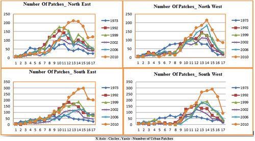
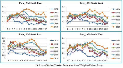
Landscape Metrics: Landscape metrics were computed circle-wise for each zones. Percentage of Landscape (PLAND) indicates that the Greater Bangalore is increasingly urbanized as we move from the centre of the city towards the periphery. This parameter showed similar trends in all directions. It varied from 0.043 to 0.084 in NE during 1973. This has changed in 2010, and varies from 7.16 to 75.93. NW also shows a maximum value of 87.77 in 2010. Largest patch index indicate that the city landscape is fragmented in all direction during 1973 due to heterogeneous landscapes. However this has aggregated to a single patch in 2010, indicating homogenisation of landscape. The patch sizes were relatively small in all directions till 2002 with higher values in SW and NE. In 2006 and 2010, patches reached threshold in all directions except NW which showed a slower trend. Largest patches are in SW and NE direction (2010). The patch density was higher in 1973 in all directions due to heterogeneous land uses, which increased in 2002 and subsequently reduced in 2010, indicating the sprawl in early 2000’s and aggregation in 2010. PAFRAC had lower values (1.383) in 1973 and maximum of 1.684 (2010) which demonstrates circular patterns in the growth evident from the gradient. Lower edge density was in 1973, increased drastically to relatively higher value 2.5 (in 2010). Clumpiness index, Aggregation index, Interspersion and Juxtaposition Index highlights that the centre of the city is more compact in 2010 with more clumpiness in NW and SW directions. Area weighted Euclidean mean nearest neighbour distance is measure of patch context to quantify patch isolation. Higher v values in 1973 gradually decrease by 2002 in all directions and circles. This is similar to patch density dynamics and can be attributed to industrialization and consequent increase in the housing sector. Analyses confirm that the development of industrial zones and housing blocks in NW and SW in post 1990’s, in NE and SE during post 2000 are mainly due to policy decision of either setting up industries or boost to IT and BT sectors and consequent housing, infrastructure and transportation facilities. PCA was performed with 21 metrics computed zonewise for each circle. This helped in prioritising the metrics (Table 2) while removing redundant metrics for understanding the urbanization, which are discussed next.

1. Number of urban patches has steadily decreased in the inner core circles from 1973 to 2010, which indicates aggregation. A sharp increase in the urban patches in the periphery (outer rings) from 25 to 120 indicates of numerous smallurban patches pointing to the urban sprawl. Urban sprawl is thus effectively visualized by this index, evident with SW, SE and NE zones in Figure 10.  The outer circle having on an average 120 urban patches compared to 5 in inner circles.

2. Perimeter Area Weighted Mean Ratio (PAWMR) reflects the patch shape complexity and is given in Figure 11. The values closer to zero in the inner circles indicate the simple shape, whereas the outer circles show the increasing trends in all directions. This highlights an enhanced rate of anthropogenic interventions and hence the process of Sprawl.

3. Landscape shape index indicates the complexity of shape, close to zero indicates maximally compact (at city centre) and higher values in  outer circles indicate disaggregated growth in 2010 (Figure 12). The trend of sprawl at city outskirts as well as at the centre was noticed till 1980’s. However, post 80’s values indicate of compactness at city centre, while outer rings show disaggregated growth.

4. Clumpiness index represents the similar trend of compact growth at the center of the city which gradually decreases towards outer rings indicating the urban agglomeration at centre and phenomena of sprawl at the outskirts in 2010 (Figure13). This phenomenon is very prominent in Northeast and Southwest direction.

5. Aggregation index indicated that the patches are maximally aggregated in 2010 while it was more dispersed in 1973, indicating that city is getting more and more compact (Figure 14).

6. Interspersion and Juxtaposition Index was very high as high as 94 in all directions which indicate that the urban area is becoming a single patch and a compact growth towards 2010 (Figure 15). All these metrics point towards compact growth in the region, due to intense urbanization.  Concentrated growth in a region has telling influences on natural resources (disappearance of open spaces – parks and water bodies), traffic congestion, enhanced pollution levels and also changes in local climate (Ramachandra and Kumar 2009; 2010)

Figure 10: Number of Patches – Direction-wise/ Circle-wise.

Figure 11: PARA_AM – Direction-wise/ Circle-wise.

Figure 12: LSI – Direction-wise/ Circle-wise.

Figure 13: Clumpiness Index – Direction-wise/ Circle-wise.

Figure 14: Aggregation Index – Direction-wise/ Circle-wise.

Figure 15: Interspersion and Juxtaposition – Direction-wise/ Circle-wise.

Note: X axis Represents Gradients taken from the center and y axis the metric value in  Figures 10 to 15.

The discussion so far highlights that the development during 1992 to 2002 was phenomenal in NW, SW due to Industrial development (Rajajinagar Industrial estate, Peenya industrial estate etc.) in these areas and subsequent housing colonies in the nearby localities. The urban growth picked up in NE and SE (Whitefield, Electronic city etc.) during post 2000 due to State’s encouraging policy to information technology and biotechnology sectors and also setting up international airport.

VI. Conclusion

Urban dynamics of rapidly urbanizing landscape – Bangalore has been analysed to understand historical perspective of land use changes, spatial patterns and impacts of the changes. The analysis of changes in the vegetation cover shows a decline from 72% (488sq.km in 1973) to 21% (145sq.km in 2010) during the last four decades in Bangalore.

Land use analyses show that there has been a 584% growth in built-up area during the last four decades with the decline of vegetation by 66% and water bodies by 74%. Temporal Analyses of Greater Bangalore reveals an increase in urban built up area by 342.83% (during 1973 to 1992), 129.56% (during 1992 to 1999), 106.7% (1999 to 2002), 114.51% (2002 to 2006) and 126.19% from 2006 to 2010. Urban growth pattern of Greater Bangalore has been done in four directions through landscape metrics and gradient analysis across six time periods. The urban density gradient illustrates radial pattern of urbanization during 1973 to 2010 indicating of intense urbanization at central core and sprawl at outskirts, which conform with Shanon’s entropy, alpha and beta population densities. Landscape metrics further highlight of compact growth in the region.

Gradients of alpha and beta densities illustrate urban intensification in the center and sprawl in NW and SW regions. Landscape metrics point towards compact growth in the region, due to intense urbanization in 2000. The analysis confirms that the nature of land use depended on the activities while the level of spatial accumulation depended on the intensity and concentration of urban builtup. Central areas have a high level of spatial accumulation and corresponding land uses, such as in the CBD, while peripheral areas have lower levels of accumulation. Unplanned concentrated growth or intensified developmental activities in a region has telling influences on natural resources (disappearance of open spaces – parks and water bodies), traffic congestion, enhanced pollution levels and also changes in the local climate.

Acknowledgement:

We are grateful to NRDMS Division, The Ministry of Science and Technology, Government of India and Centre for infrastructure, Sustainable Transportation and Urban Planning (CiSTUP), Indian Institute of Science for the financial and infrastructure support.

VII. References

1. Angel, S., Parent, J., Civco, D., 2007. Urban sprawl metrics: an analysis of global urban expansion using GIS. Proceedings of ASPRS 2007 Annual Conference, Tampa, Florida May 7–11. URL: http://clear.uconn.edu/publications/research/tech_papers/Angel_et_al_ASPRS2007.pdf
2. Barredo, J.l., Demicheli,  L., 2003.  Urban sustainability in developing countries mega cities, modeling  and  predicting  future  urban  growth  in lagos. Cities, 20(5): 297-310.
3. Bhatta, B., 2009a. Analysis of urban growth pattern using remote sensing and GIS: a case study of Kolkata, India. International Journal of Remote Sensing, 30(18):4733–4746.
4. Bhatta, B., 2009b. Modeling of urban growth boundary using geoinformatics. International Journal of Digital Earth, 2(4):359–381.
5. Bhatta, B., 2010. Analysis of urban growth and sprawl from remote sensing data. Berlin, Heidelberg: Springer-Verlag.
6. Brueckner, J. K., 2000. Urban Sprawl: Diagnosis and remedies. International Regional Science Review, 23(2), 160–171.
7. Chen, S., Zeng, S., Xie, C., 2000. Remote Sensing and GIS for urban growth analysis in China. Photogrammetric Engineering and Remote Sensing, 66(5), 593–598.
8. Congalton, R. G., Oderwald, R. G., Mead, R. A., 1983. Assessing Landsat classification accuracy using discrete multivariate analysis statistical techniques. Photogrammetric Engineering and Remote Sensing, 49, 1671−1678.
9. Crews-Meyer, K.A., 2002. Characterizing landscape dynamism using paneled-pattern metrics. Photogrammetric Engineering and Remote Sensing, 68(10), 1031-1040. 
10. Dietzel, C., Herold, M., Hemphell,  J.J., Clarke, K.C.,  2005.  Spatio-temporal  dynamics  in  California's central  valley: Empirical  links  to urban  theory. Int. J. Geographic Information Science,  19(2): 175-195.
11. Duda, R.O., Hart, P.E., Stork, D.G., 2000, Pattern Classification, A Wiley-Interscience Publication, Second Edition, ISBN 9814-12-602-0.
12. Epstein, J., Payne, K., Kramer, E., 2002. Techniques for mapping suburban sprawl. Photogrammetric Engineering and Remote Sensing, 63(9), 913 – 918.
13. Galster G., Hanson R., Ratclfee., M R, 2001. Wrestling sprawl to the ground: Defining and measuring an elusive concept, Housing Policy Debate, 12(4):681-717
14. Gao., Y. Liu, 2008. Mapping land degradation from space: A comparative study of Landsat ETM+ and ASTER data. International Journal of Remote Sensing, 29, 4029–4043.
15. Geri, F., Amici, V., Rocchini, D., Human activity impact on the heterogeneity of a Mediterranean landscape. Applied Geography, doi:10.1016/j.apgeog.2009.10.006, (in press).
16. Gustafson,  E.J., 1998. Quantifying landscape spatial pattern: what is the state of the art?, Ecosystems 1, 143–156.
17. Herold, M., Goldstein, N., C., Clarke, K., C., 2003. The spatiotemporal form of urban growth: measurement, analysis and modeling. Remote Sensing of the Environment, 86, 286–302.
18. Herold, M., Scepan, J.,  Clarke, K. C., 2002. The use of remote sensing and landscape-metrics to describe structures and changes in urban land uses. Environment and Planning , 34, 1443–1458.
19. Huang J, Lu X, Sellers J., 2007. A Global comparative analysis of urban form: Applying spatial metrics and remote sensing, Landscape and Urban Planning, 82(4):184-197
20. Hulshoff, R. M., 1995. Landscape indices describing a Dutch landscape, Lands. Ecol. 10(2), 101–111.
21. Janssen L.L.E, 2000. Principles of remote sensing, First Edition, The international institute for Aerospace Survey and Earth Science(ITC). ISBN 90-61-64-183-7:132-133.
22. Ji, C. Y., Lin, P., Li, X., Liu, Q., Sun, D.,  Wang, S., 2001. Monitoring urban expansion with remote sensing in China. International Journal of Remote Sensing, 22(8), 1441–1455.
23. Ji, W., Ma, J,  Twibell R. W., Underhill, K., 2006. Characterizing urban sprawl using multi-stage remote sensing images and landscape metrics, Computers, Environment and Urban Systems, 30, 861–879.
24. Jiang, F., Liu, S., Yuan, H., Zhang, Q., 2007. Measuring urban sprawl in Beijing with geo-spatial indices, Journal of Geographical Sciences, 17, 469-478.
25. Jim, C.Y.. and Chen, W.Y., 2009. Diversity and distribution of landscape trees in the compact Asian city of Taipei, Applied Geography, 29(4), 577–587.
26. Kienast, F., 1993, Analysis of historic landscape patterns with a Geographical Information System – a methodological outline, Lands. Ecol. 8(2), 101–118.
27. Lata, K.M., Rao, C.H.S., Prasad, V.K.,  Badarianth, K.V.S.,  Raghavasamy,  V., 2001. Measuring  Urban sprawl' A case study of Hyderabad, gis@development, 5(12), 26-29.
28. Lausch, A., Herzog, F., 1999. Applicability of landscape metrics for the monitoring of landscape change: issues of scale, resolution and interpretability. Paper presented at the International Conference, in St.-Petersburg, Russia.
29. Li,  X., Yeh,  A.G.O., 2004.  Analyzing  spatial restructuring  of landuse  patterns  in a  fast growing region  remote  sensing  and  GIS. Landscape  and Urban  planning, 69, 335-354.
30. Lillesand, T.M., Kiefer. R. W., 2002. Remote Sensing and Image Interpretation, Fourth Edition, John Wiley and Sons, ISBN 9971-51-427-3.Pages:215-216
31. Lo, C.P., Yang, X., 2002. Drivers of land-use/land-cover changesand dynamic modelling for the Atlanta, Georgia MetropolitanArea. Photogrammetr. Eng. Remote Sens. 68(10), 1062–1073.
32. Lucy w. and Philips D., 2001. Suburbs and the Census: Patterns of Growth and Decline, Survey Series, Washington D C: Brookings Instituition, Centre on Urban and Metropolitan Policy
33. Luque, S. S., Lathrop, R. G., Bognar, J. A., 1994, Temporal and spatial changes in an area of the New Jersey Pine landscape, Lands. Ecol. 9(4), 287–300.
34. McGarigal, K., & Marks, B. J., 1995. FRAGSTATS: spatial pattern analysis program for quantifying landscape structure. USDA Forest Service General Technical Report PNW-351.
35. Medley, K. E., Okey, B. W., Barrett, G. W., Lucas, M. F., Renwick, W. H., 1995, Landscape change with agricultural intensification in a rural watershed, southwestern Ohio, U.S.A., Lands. Ecol. 10(3), 161–176.
36. Mitrakis, N. E., Topalogou, C. A., Alexandridis, T. K., Theocharis, J. B., Zalidis, G. C., 2008. A novel self organising neuro-fuzzy multilayered classifier for land cover classification of a VHR image. International Journal of Remote Sensing, 29, 4061− 4087.
37. Ngigi, T. G., Tateishi, R., Shalaby, A., Soliman, N., Ghar, M., 2008. Comparison of a new classifier, The mix unmix classifier, with conventional hard and soft classifiers. International Journal of Remote Sensing, 29, 4111 −4128.
38. Palang, H., Mander, Ü., Luud, A., 1998. Landscape diversity changes in Estonia, Lands. and Urban Plann. 41, 163–169.
39. Pan, D., Domon, G., de Blois, S., Bouchard, A.: 1999, ‘Temporal (1958–1993) and spatial patterns of land use changes in Haut-Saint-Laurent (Quebec, Canada) and their relation to landscape physical attributes’, Lands. Ecol. 14, 35–52.
40. Pathan,  S.K.,  Patel,  J  G.,  Bhanderi.  R.J.,  Ajai, Kulshrestha,  Goyal,  V.P., Banarjee.  D.L.,  Marthe, S., Nagar, V.K.,  Katare, V., 2004.  Urban planning with  specific rel;erence to master plan of lndore city using  RS  and  GIS  techniques.  Proc.  of GSDI-7 International  Conference  on  Spatial  Data Infrastructure  for Sustainable  Development,  held  at Bangalore from Feb, 2-6, 2004.
41. Pathan,  S.K.,  Sampat Kumar D., Mukund Rao., Sastry S.V.C., 1993. Urban  growth  trend  analysis  using GIS  techniques-A  case  study  of  the  Bombay Metropolitan  Region.,  Int. J  Remote Sensing,  14(17), 3169 - 3179
42. Pathan,  S.K., Shukla, V.K., Patel,  R.G., Mehta,  K,S., 1991. Urban  land  use mapping  - A case study of Ahmedabad  city  and  its  environs.  J  Indian  Soc Remote Sensing,  19(2), 95- I 12.
43. Pathan, S.K., Jothimani, P., Pendharkar, S.P. and Sampat Kumar,  D., 1989.  Urban  land  use mapping and zoning  of Bombay Metropolitan  Region  using Remote Sensing data. J. Indian Soc. Remote Sensing, 17(3), 11-22.
44. Peiser, R., 2001. Decomposing urban sprawl. Town Planning Review, 72(3), 275–298.
45. Rainis, R., 2003. Application of GIS and landscape metrics in monitoring urban land use change. In N. M. Hashim, & R. Rainis (Eds.), Urban ecosystem studies in Malaysia: A study of change, 267 – 278.
46. Ramachandra T. V., Kumar, U., 2008. Wetlands of Greater Bangalore,  India: Automatic Delineation  through  Pattern  Classifiers.  Electronic Green  Journal,  Issue 26, Spring 2008 ISSN: 1076-7975.
47. Ramachandra, T. V., Kumar, U., 2009. Land surface temperature with land cover dynamics: multi-resolution, spatio-temporal data analysis of Greater Bangalore, International Journal of Geoinformatics, 5 (3), 43-53
48. Ramachandra, T. V., Kumar, U., 2010. Greater Bangalore: Emerging Heat Island, GIS for Development, 14(1): 86-104 http://www.gisdevelopment.net/application/urban/sprawl/Greater-Bangalore-Emerging-Urban-Heat-Island.htm
49. Sachs, D. L., Sollins, P., Cohen, W. B., 1998. Detecting landscape changes in the interior of British Columbia from 1975 to 1992 using satellite imagery, Can. J. Forest Res. 28, 23–36.
50. Sha, Z., Bai, Y., Xie, Y., Yu, M.,  Zhang, L., 2008. Using a hybrid fuzzy classifier (HFC) to map typical grassland vegetation in Xilin River Basin, Inner Mongolia, China. International Journal of Remote Sensing, 29, 2317−2337.
51. Simpson, J. W., Boerner, R. E. J., DeMers, M. N., Berns, L. A., 1994, Forty-eight years of landscape change on two contiguous Ohio landscapes, Lands. Ecol. 9(4), 261–270
52. Sudhira H.S.,  Ramachandra T.V.,  Bala Subramanya M.H., 2007.  City Profile:  Bangalore.,  Cities l24(4), 379-390.
53. Sudhira,  H.S.,  Ramachandra,  T.V.,  and  Jagadish,  K.S., 2004.  Urban  sprawl:  metrics,  dynamics  and modelling  using  G1S.  Int.  J  Applied  Earth Observation and Geoinformation,  5, 29-39.
54. Thibault, P. A. and Zipperer, W. C., 1994, Temporal changes of wetlands within an urbanizing agricultural landscape, Lands. and Urban Plann. 28, 245–251.
55. Tian, G., Liu, J., Xie, Y., Yang, Z., Zhuang, D., and Niu, Z. 2005. Analysis of spatio temporal dynamic pattern and driving forces of urbanland in China in 1990s using TM images and GIS. Cities 22(6), 400-410.
56. Torrens P. M., and Alberti M., 2000. Measuring sprawl. Working paper no. 27, Centre for Advanced Spatial Analysis, University College, London.
57. Turner, M.G., Gardner R.H., O'Neill, R.V., 2001. Landscape ecology in theory and practice: Pattern and process, Springer, New York.
58. Wang F., 2009. Factor Analysis and Principal-Components Analysis. International Encyclopedia of Human Geography. doi:10.1016/B978-008044910-4.00434-X.
59. World Urbanization Prospects, 2005, Revision, Population Division, Department of Economic and Social Affaris, UN.
60. Yeh,  A.G.O., and  Liu,  X.,  2001.  Measurement  and Monitoring  of urban  sprawl  in  a Rapidly growing region using Entropy, Photogramm  Engg & Remote Sensing,  67(I),  83-90.
61. Yu, X. J., and Ng, C. N. 2007. Landscape and urban planning. Spatio and temporal dynamics of urban sprawl along two urban-rural transects: A case study of Guamgzhou, China 79, 96-109.
62. Zhang, Q., Wang, J.,  Peng,  X., Gang, R., Shi, P., 2002. Urban  built-up  land  change  detection  with  road density  and  spectral  information  from  multi- temporal  Landsat TM  data.  Int.  J.  Remote Sensing, 23(15), 3057-3078.
63. Zheng, D., Wallin, D. O. and Hao, Z., 1997. Rates and patterns of landscape change between 1972 and 1988 in the Changbai Mountain area of China and North Korea,  Lands. Ecol. 12, 241–254.
    

Back

Top

Next