|
Indicators |
Formula |
Range |
Significance/
Description |
| Category : Patch area metrics |
| 1 |
Built up (Total Land
Area) |
------ |
>0 |
Total built-up land
(in ha) |
| 2 |
Percentage of
Landscape
(PLAND) |
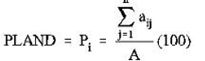
Pi = proportion of the landscape
occupied by patch type
(class) i.
aij = area (m2) of patch ij.
A = total landscape area (m2). |
0 <
PLAND ≤
100 |
PLAND
approaches 0
when the
corresponding
patch type (class)
becomes
increasingly rare
in the landscape.
PLAND = 100
when the entire
landscape consists
of a single patch
type; |
| 3 |
Largest Patch
Index (Percenta
ge of
landscape) |
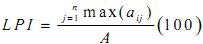
a ij = area (m2) of patch ij
A= total landscape area |
0 ≤
LPI≤100 |
LPI = 0 when
largest patch of
the patch type
becomes
increasingly
smaller.
LPI = 100 when
the entire
landscape consists
of a single patch
of, when the
largest patch
comprise 100% of
the landscape |
| 4 |
Number of
Urban Patches |
N P U = n
NP equals the number of patches
in the landscape. |
NPU>0,
without
limit. |
It is a
fragmentation
Index. Higher the
value more the
fragmentation |
| 5 |
Patch
density |
f(sample area) = (Patch
Number/Area) * 1000000 |
PD>0, without limit |
Calculates patch
density index on a
raster map, using
a 4 neighbor
algorithm. Patch
density increases
with a greater number of patches
within a reference
area. |
| 6 |
Perimeter-Area Fractal
Dimension
PAFRAC |
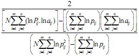
Perimeter-Area Fractal Dimension
aij = area (m2) of patch ij.
pij = perimeter (m) of patch ij.
N = total number of patches in
the landscape |
1 ≤ PAFRAC ≤ 2 |
It approaches 1
for shapes with
very simple
perimeters such as
squares, and
approaches 2 for
shapes with highly
convoluted,
perimeters.
PAFRAC requires
patches to vary in
size. |
| 7 |
Landscape
Division Index
(DIVISION) |
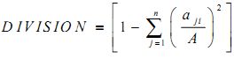
a ij = area (m2) of patch ij
A= total landscape area |
0≤DIVISION<1 |
DIVISION =
0, when the
landscape consists
of single patch. It
approaches 1
when the
proportion of
landscape
comprising of the
focal patch type
decreases and as
those patches
decreases in size. |
| Category : Edge/border metrics |
| 8 |
Edge density |
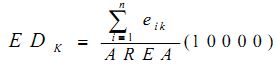
k: patch type
m: number of patch type
n: number of edge segment of patch
type k
eik :total length of edge in
landscape involving patch type k
Area: total landscape area |
ED ≥ 0,
without
limit. ED =
0 when
there is no
class edge. |
ED measures
total edge of
urban boundary
used to compare
landscape of
varying sizes. |
| 9 |
Area weighted
mean patch
fractal
dimension
(AWMPFD) |
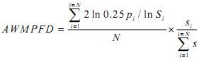
Where si and pi are the area and
perimeter of patch i, and N is the
total number of patches |
1 ≤ AWMPFD ≤ 2 |
AWMPFD
approaches 1 for
shapes with very
simple
perimeters, such
as circles or
squares, and
approaches 2 for
shapes with highly
convoluted
perimeter
AWMPFD
describes the
fragmentation of
urban patches. If
Sprawl is high
then the
AWMPFD value
is high |
| 10 |
Perimeter Area
Weighted Mean
Ratio.
PARA_AM |
PARA _AM= Pij/Aij
Pij = perimeter of patch ij
Aij= area weighted mean of patch ij
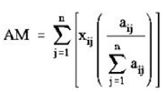 |
≥ 0,
without
limit |
PARA AM is a
very useful
measure of
fragmentation; it
is a measure of
the amount of
'edge' for a
landscape or
class. PARA AM
value increased
with increasing
patch shape
complexity,
which precisely
characterized the
degree of patch
shape
complexity. |
| 11 |
Mean Patch
Fractal
Dimension
(MPFD) |
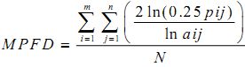
pij = perimeter of patch ij
aij= area weighted mean of patch ij
N = total number of patches in
the landscape |
1<=MPFD<2 |
Shape
Complexity.
MPFD is another
measure of shape
complexity,
approaches one
for shapes with
simple
perimeters and
approaches two
when shapes are
more complex. |
| 12 |
Total Edge
(TE) |
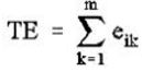
eik = total length (m) of edge in
landscape involving patch
type (class) i; includes
landscape boundary and
background segments
involving patch type i. |
TE>0,
Without
limit |
TE equals the
sum of the
lengths (m) of all
edge segments
involving the
corresponding
patch type. TE
includes a user-specified
proportion of
internal
background edge
segments
involving the
corresponding
patch type |
| Category : Shape metrics |
| 13 |
NLSI(Normalized Landscape
Shape Index) |
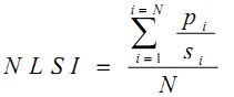
Where si and pi are the area and
perimeter of patch i, and N is the
total number of patches. |
0≤NLSI<1 |
NLSI = 0 when
the landscape
consists of single
square or
maximally
compact almost
square, it
increases when
the patch types
becomes
increasingly
disaggregated
and is 1 when the
patch type is
maximally
disaggregated |
| 14 |
Landscape
Shape Index
(LSI) |
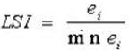
ei = total length of edge (or
perimeter) of class i
in terms of number
of cell surfaces;
includes all
landscape boundary
and background edge
segments involving
class i.
min ei = minimum total length of
edge (or perimeter)
of class i in terms of
number of cell surfaces (see below). |
LSI>1,
Without
Limit |
LSI = 1 when the
landscape
consists of a
single square or
maximally
compact (i.e.,
almost square)
patch of the
corresponding
type; LSI
increases without
limit as the patch
type becomes
more
disaggregated |
| Category: Compactness/ contagion / dispersion metrics |
| 15 |
Clumpiness |
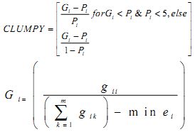
gii =number of like adjacencies
(joins) between pixels of patch type
(class) I based on the double-count
method.
gik =number of adjacencies (joins)
between pixels of patch types
(classes) i and k based on the
double-count method.
min-ei
=minimum perimeter (in number of
cell surfaces) of patch type (class)i
for a maximally clumped class.
Pi =proportion of the landscape
occupied by patch type (class) i. |
-1≤
CLUMPY
≤1 |
It equals 0 when
the patches are
distributed
randomly, and
approaches 1
when the patch
type is
maximally
aggregated |
| 16 |
Percentage of
Like
Adjacencies
(PLADJ) |
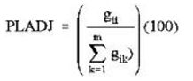
gii = number of like adjacencies
(joins) between pixels of
patch type (class) i based on
the double-count method.
gik = number of adjacencies
(joins) between pixels of
patch types (classes) i and k
based on the double-count
method. |
0<=PLADJ<=100 |
The percentage
of cell
adjacencies
involving the
corresponding
patch type that
are like
adjacencies. Cell
adjacencies are
tallied using the
double-count
method in which
pixel order is
preserved, at
least for all
internal
adjacencies |
| 17 |
Total Core
Area (TCA) |
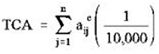 |
TCA>=0
Without
limit. |
TCA equals the
sum of the core
areas of each
patch (m2) of the
corresponding
patch type, divided by
10,000 (to
convert to
hectares). |
| 18 |
ENND
coefficient of
variation |
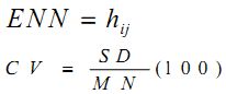
CV (coefficient of variation) equals
the standard deviation divided by
the mean, multiplied by 100 to
convert to a percentage, for the
corresponding patch metrics. |
It is
represented
in
percentage. |
In the analysis of
urban processes,
greater isolation
indicates greater
dispersion. |
| 19 |
Aggregation
index |
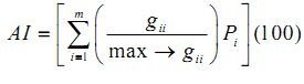
gii =number of like adjacencies
(joins) between pixels of patch type
(class) i based on the single count
method.
max-gii = maximum number of like
adjacencies (joins) between pixels
of patch type class i based on single
count method.
Pi= proportion of landscape
comprised of patch type (class) i. |
1≤AI≤100 |
AI equals when
the patches are
maximally
disaggregated
and equals 100
when the patches
are maximally
aggregated into a
single compact
patch.
Aggregation
corresponds to
the clustering of
patches to form
patches of a
larger size. |
| 20 |
Interspersion
and
Juxtaposition |
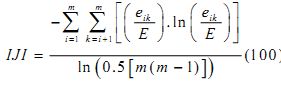
eik = total length (m) of edge in
landscape between patch types
(classes) i and k.
E = total length (m) of edge in
landscape, excluding background
m = number of patch types
(classes) present in the landscape,
including the landscape border, if
present. |
0≤ IJI ≤100 |
IJI is used to
measure patch
adjacency. IJI
approach 0 when
distribution of
adjacencies
among unique
patch types
becomes
increasingly
uneven; is equal
to 100 when all
patch types are
equally adjacent
to all other patch
types. |