MATERIALS AND METHOD

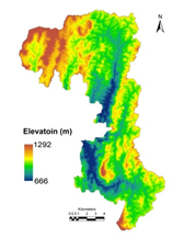
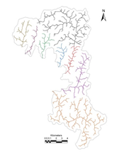
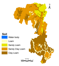
2.1 Study area: Yettinaholé catchment has a pristine ecosystem with rich biodiversity (Figure 1 and Table 1), extend from 12044’N to 12058’N Latitude and 75037’E to 75047’E longitude encompassing total area of 179.68 km2. The terrain (Figure 2) is undulating with altitude varying from 666m above MSL to 1292m above MSL leading to higher density of stream network (Figure 3). Geologically, rock types consist of Gneiss, the soils are loamy ranging from sandy loamy to clay loamy. Soils (Figure 4) in the region are fertile and highly permeable, hence allowing the precipitated water to percolate easily into the subsurface recharging ground water and storing water in the sub surfaces and hence keeping the water source perennial to the catchment and the downstream users during and post monsoon.
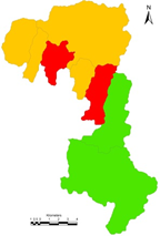
Decadal population in Sakleshpura taluk (spatial extent 1034 sq. km) of Hassan district is given in Figure 5 and Table 2 shows a declining trend due to migration to cities during post 2001. Population dynamics of the catchments also follows the dynamics of Sakleshpura taluk. Total Population of all the catchments with respect to census data [24, 25] was estimated as 17005 in 2001, has declined to 16345 in 2011 at a decadal rate of 3.88%. Population for the year 2014 was calculated as 16156 based on the temporal data. Population density for each of the sub catchments are as depicted in Figure 6 and Table 3.

Table 1: Study Area

Table 2: Population Growth of Sakleshpura Taluk [24, 25]

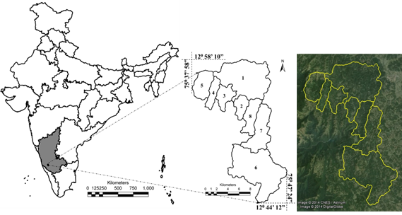
Figure 1: Study Area – Yettinaholé catchment, Karnataka, India

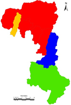
Figure 2: Digital Elevation Model	Figure 3: Stream Network	Figure 4: Soil

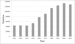
Figure 5: Population Growth of Sakleshpura Taluk

Figure 6: Population Density in Sub Catchments

Table 3: Population density (persons per sq.km)

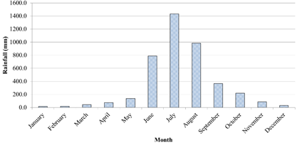
Figure 7: Rainfall in mm

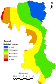
Figure 8: Rainfall distribution

The region receives an annual rainfall of 3500 to 5000 mm across the catchment. Precipitation in the catchment during June to September is due to the southwest monsoons, with July having maximum rainfall over 1300 mm. Monthly variation in rainfall is depicted in Figure 7. Spatial variation of rainfall across the catchments was assessed based on 110 years data [26] (1901 to 2010) from the rain gauge stations in and around the catchment (Figure 8). Figure 9 depicts monthly temperatures [27] variations,  which ranges from 14.7 °C (January) to  31.6 °C (in March).

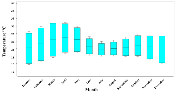
Figure 9: Monthly temperature variations

2.2 Data: Data required for hydrological and land use analyses were (i) social and demographic data from the government agencies, (ii) temporal remote sensing data from public archive and (iii) primary data through field investigations. Latest remote sensing data used is of Landsat 8 series (2014). Rainfall data was acquired from the Directorate of Economics and Statistics, Government of Karnataka [26], Temperature data was sourced from World Clim-Global Climate Data [27] of 1km resolution. Census data collected from government of India, state and district census departments [24, 25]. These data was supplemented with secondary data compiled from various sources as tabulated in Table 4. Primary data is compiled through field investigations and through structured questionnaire (household survey).

Table 4: Data used for land use and assessment of hydrologic regime

2.3 Method: The method for the evaluation of the environmental flow and hydrological status is given in Figure 10. Hydrologic assessment in the catchment involved 1) delineation of catchment boundary 2) land use analysis, 3) assessment of the hydro meteorological data, 4) analysis of population census data, 5) compilation of data through public interactions for assessing the water needs for livestock, agriculture/horticulture and cropping pattern, and 6) evaluation of hydrologic regime.

2.3.1 Delineation of catchment boundary: Catchment boundaries (Figure 1) and the stream networks (Figure 3) were delineated considering the topography of the terrain based on CartoSat DEM using the QSWAT module – Quantum GIS 2.10 32bit. These catchment boundaries were overlaid on the extracted boundaries from the Survey of India topographic maps for validations. Corrected catchment boundaries were further overlaid on Google earth in order to visualize the terrain variations (Figure 2).

Figure 10: Method for computing environmental flow based on hydrologic variables

2.3.2 Land use Assessment: Large scale land-use land-cover (LULC) changes leading to deforestation is one of the drivers of global climate changes and alteration of biogeochemical cycles. This has given momentum to investigate the causes and consequences of LULC by mapping and modelling landscape patterns and dynamics and evaluating these in the context of human-environment interactions in the riverine landscapes. Human induced environmental changes and consequences are not uniformly distributed over the earth. However their impacts threaten the sustenance of human-environmental relationships. Land cover refers to physical cover and biophysical state of the earth’s surface and immediate subsurface and is confined to describe vegetation and manmade features. Thus, land cover reflects the visible evidence of land cover of vegetation and non-vegetation. Land use refers to use of the land surface through modifications by humans and natural phenomena. Heterogeneous terrain in the landscape with the interacting ecosystems is characterized by its dynamics. Human induced land use and land cover (LULC) changes have been the major driver of the landscape dynamics at local levels. Land use assessment was carried using the maximum likelihood classification technique [48, 49]. Understanding of landscape dynamics helps in the sustainable management of natural resources.
Land use analysis involved i) generation of FCC- False Colour Composite (Figure 11) of remote sensing data (bands – green, red and NIR). This helped in locating heterogeneous patches in the landscape ii) selection of training polygons (these correspond to heterogeneous patches in FCC) covering 15% of the study area and uniformly distributed over the entire study area, iii) loading these training polygons co-ordinates into pre-calibrated GPS, vi) collection of the corresponding attribute data (land use types) for these polygons from the field. GPS helped in locating respective training polygons in the field, iv) supplementing this information with Google Earth  v) 65% of the training data has been used for  classification, while the balance is used for validation or accuracy assessment.
Land uses were categorized into 8 classes namely. i) water bodies (lakes/tanks, rivers, streams, ii) built up (buildings, roads or any paved surface, iii) open spaces iv) evergreen forest (evergreen and semi evergreen), v) deciduous forest (Moist deciduous and dry deciduous) vi) scrub land and grass lands, vii) agriculture, (viii) private plantations (coconut, arecanut, rubber) and) forest plantations (Acacia, Teak, etc.)

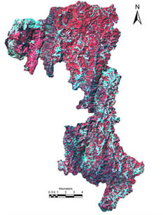
Figure 11: False Colour Composite of Study area

2.3.3 Assessment of the hydro meteorological data: This involved assessment of the spatial and temporal variations in rainfall [26, 29, 50] in and around the study region. Long term precipitation data helped in understanding the rainfall variability over decades. Along with rainfall, temperature (minimum, maximum and average), extra-terrestrial solar radiation across the catchment were used to hydrological behaviors of the catchments which enables to understand the hydrological status.
Rainfall: Point data of daily rainfall from rain gauge stations for the period 1901- 2010 [26, 29, 50] were used for the analysis. Some rain gauge stations had incomplete records with missing data for few months.  The average monthly and annual rainfall data were used to derive rainfall map throughout the study area and was used to derive the gross yield (RG) in the basin (equation 1). Net yield (RN) was quantified (equation 2) as the difference between gross rainfall and interception (In).
RG = A * P ……. (1)
RN = RG – In …… (2)
Where, RG :   Gross rainfall yield volume; A:   Area in Hectares; P:  Precipitation in mm, RN:  Net rainfall yield volume;  and      In:  Interception volume

Interception: During monsoons, portion of rainfall does not reach the surface of the earth; it remains on the canopy of trees, roof tops, etc. and gets evaporated. Field studies in Western Ghats show that, losses due to interception is about 15% to 30%, based on the canopy cover. Table 5 shows the interception loss across various rainy months and land uses.

Table 5: Interception loss

Runoff: Portion of rainfall that flows in the streams after precipitation [2, 8, 10, 11] are  (i) surface runoff or direct runoff  and (ii) sub surface runoff. 
Surface runoff: Portion of water that directly enters into the streams during rainfall, which is estimated based on the empirical [9, 10, 11] relationships given in equation 3.
Q = Σ(Ci*PR*Ai)/1000 ……(3)
Where, Q : Runoff in cubic meters per month; C : Catchment / Runoff coefficient, depends on land uses as given in Table 6 [36];  PR : Net rainfall in mm;       i : Land use type; Ai : Area of Landscape i as square meters.

Table 6: Catchment coefficients

Infiltration: The portion of water enters the subsurface (vadoze and groundwater zones) during precipitation depending on land cover in the catchment. During field monitoring of streams in the forested catchment, overland flow is noticed in streams only after  couple of days rainfall. This means that overland flow in the catchment with vegetation cover happens after the saturation of sub surfaces. The water stored in sub-surfaces will flow laterally towards streams and contributes to stream flow during non-monsoon periods, which are referred as pipe flow (during post monsoon) and base flow (during summer).
Inf = RN – Q ……(4)
Ground water recharge: This is the portion of water that is percolated below the soil stratum (vadoze) after soil gets saturated. Recharge is considered the fraction of infiltrated water that recharges the aquifer after satisfying available water capacity and pipe flow. Krishna Rao equation, (equation 5) [19] was used to determine the ground water recharge. 
GWR = RC * (PR – C) * A ……(5)
Where, GWR  : Ground water recharge; RC: Ground water recharge coefficient (Table 7); C: Rainfall Coefficient (Table 7);  A: Area of the catchment. The recharge coefficient and the constant vary depending land uses with the annual rainfall.

Table 7: Ground water recharge coefficients

Sub Surface Flow (Pipe flow): Part of the infiltrated effective rainfall circulates more or less horizontally (lateral flow) in the superior soil layer and appears at the surface through stream channels is referred as subsurface flow. The presence of a relatively permeable shallow layer favors this flow. Subsurface flows in water bearing formations have a drainage capacity slower than superficial flows, but faster than groundwater flows. Pipe flow is considered to be the fraction of water that remains after infiltrated water satisfies the available water capacities under each soil. Pipe flow is estimated for all the basins as function of infiltration, ground water recharge and pipe flow coefficient, given by equation 6
PF = (Inf – GWR) * KP ……. (6)
Where, PF : Pipeflow; Inf: Infiltration volume; KP: Pipe flow coefficient [2]

Groundwater Discharge: Groundwater discharge or base flow is estimated by multiplying the average specific yield of aquifer under each land use with the recharged water. Specific yield represents the water yielded from water bearing material. In other words, it is the ratio of the volume of water that the material, after being saturated, will yield by gravity to its own volume. Base flow appears after monsoon and receding of pipe-flow. This water generally sustains flow in the rivers during dry seasons. A portion of recharged water flows to the streams as ground water discharge which is dependent on the topography, geology and the land use conditions. Equation 7 defines Ground water discharge as product of specific yield and the portion of ground water recharged.
GWD = GWR * YS …… (7)
Where, GWD:  Ground water discharge; GWR:  Ground water recharge; YS: Specific yield [2].

2.3.4  Estimation of Water Demand
Evapotranspiration: Evaporation is a process where in water is transferred as vapour to the atmosphere. Transpiration is the process by which water is released to the atmosphere from plants through leaves and other parts above ground. Evapotranspiration is the total water lost from different land use due to evaporation from soil, water and transpiration by plants. . Some of the important factors that affect the rate of evapotranspiration are: (i) temperature, (ii) wind, (iii) light intensity, (iv) Sun light hours, (v) humidity, (vi) plant characteristics, (vii) land use type and (viii) soil moisture.  If sufficient moisture is available to completely meet the needs of vegetation in the catchment, the resulting evapotranspiration is termed as potential evapotranspiration (PET). The real evapotranspiration occurring in specific situation is called as actual evapotranspiration (AET). These evapotranspiration rates from forests are more difficult to describe and estimate than for other vegetation types.
Potential evapotranspiration (PET) was determined using Hargreaves method (Hargreaves, 1972 [2, 36]) an empirical based radiation based equation, which is shown to perform well in humid climates. PET is estimated as mm using the Hargreaves equation is given by equation 8.
PET = 0.0023 * (RA/λ) *  *  …… (8)
Where, RA: Extra-terrestrial radiation (MJ/m2/day) [36]; Tmax: Maximum temperature [42]; Tmin:  Minimum temperature [42]; λ: latent heat of vapourisation of water (2.501 MJ/kg)
Actual evapotranspiration is estimated as a product of Potential evapotranspiration (PET) and Evapotranspiration coefficient (KC) (table 8), given in equation 9. The evapotranspiration coefficient is a function of land use varies with respect to different land use. Table 8 gives the evapotranspiration coefficients for different land use
AET = PET * KC ……(9)

Table 8: Evapotranspiration coefficient

Note: the crop water requirement was estimated for different crops and different seasons based on land use, assumption is individual crop water requirement and different growth phases (need different quantum of water for their development inclusive of evaporation).

Domestic water demand: Understanding the population dynamics in a region is necessary to quantify and also to predict the domestic water demand. Population census for villages during 2001 and 2011 [24] were considered in order to compute the population of the basin level. Based on the rate of change of population (equation 10), the population for the year 2014 was predicted as given in equation 11.
r = (P2011/P2001 – 1)/n ……(10)
Where, P2001 and P2011 are population for the year 2001 and 2011 respectively; n is the number of decades which is equal to 1; r is the rate of change
P2014 = P2011 * (1 + n*r) ……(11)
Where, P2014 is the population for the year 2014; n is the number of decades which is equal to 0.3
Domestic water demand is assessed as the function of water requirement per person per day, population and season. Water required per person include water required for bathing, washing, drinking and other basic needs. Water requirements across various seasons are as depicted in Table 9.

Table 9: Seasonal water requirement

Livestock water requirement: Household surveys were conducted with the structured questionnaires to understand the agricultural and horticulture cropping pattern and water needed for various crops in the catchment. Livestock population details were obtained from the district statistics office and water requirement for different animals were quantified based on the household interviews. Table 10 gives the water requirement for various animals.

Table 10: Livestock water requirement

Crop water requirement: The crop water requirement for various crops was estimated considering their growth phase and details of the cropping pattern in the catchment (based on the data compiled from household surveys and publications such as the district at a glance, department of agriculture). Land use information was used in order to estimate the cropping area under various crops. Figure 12 provides the information of various crop water requirements based on their growth phase as cubic meter per hectare.

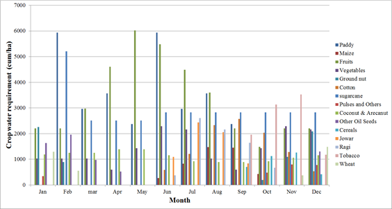
Figure 12: Crop water requirement (as cum per hectare per month)

2.3.5 Evaluating Hydrological Status: The hydrological status in the catchment is analysed for each month based on the water balance which take into account the water available to that of the demand. The water available in the catchment is function of water in the soil, run off (streams and river) and water available in the water bodies (Lentic water bodies such as lakes, etc.). Water demand in the catchment is estimated as the function of societal demand and terrestrial ecosystem (AET from forested landscape) crop water demand, domestic and livestock demand and the evapotranspiration. The catchment is considered hydrological sufficient, if the water available caters the water demand completely else the deficit catchment, if the water demand is more than the water available in the system.  
2.3.6 Quantification of the Environmental Flow: Ecological investigations include the investigations of fish diversity across seasons. Habitat simulation method [55, 56] was adopted to assess flows on basis of quantity and suitability of physical habitat available to target species under different flow regimes. In order to evaluate the natural flow regime [53, 54], 18-24 months field monitoring of select streams in Sharavathi river basin and at Hongadahalla and Kadumanehalla (of Yettinaholé catchment) was carried out. This field data was compared with the long term flow measurements data at Hongadahalla and Kadumanehalla [45].  The natural flow that sustains native biota during lean season is accounted as the ecological or environmental flow [57 - 61] for the respective lotic system. In the current study, hydrologic assessment and investigations on the occurrence of native fish species (with diversity) helped in ascertaining the minimum flow required to sustain the native fish biota.