|
Data analysis involved
1. Pre-processing: The remote sensing data obtained were geo-referenced, rectified and cropped pertaining to the study area. Geo-registration of remote sensing data (Landsat data) has been done using ground control points collected from the field using pre calibrated GPS (Global Positioning System) and also from known points (such as road intersections, etc.) collected from geo-referenced topographic maps published by the Survey of India. The Landsat satellite 1973 images have a spatial resolution of 57.5 m x 57.5 m (nominal resolution) were resampled to 28.5m comparable to the 1989 - 2010 data which are 28.5 m x 28.5 m (nominal resolution). Landsat ETM+ bands of 2010 were corrected for the SLC-off by using image enhancement techniques, followed by nearest-neighbour interpolation.
2. Vegetation Cover Analysis: Normalised Difference Vegetation index (NDVI) was computed to understand the changes in the vegetation cover during the study period. NDVI is the most common measurement used for measuring vegetation cover. It ranges from values -1 to +1. Very low values of NDVI (-0.1 and below) correspond to soil or barren areas of rock, sand, or urban builtup. Zero indicates the water cover. Moderate values represent low density vegetation (0.1 to 0.3), while high values indicate thick canopy vegetation (0.6 to 0.8).
3. Land use analysis: The method involves i) generation of False Colour Composite (FCC) of remote sensing data (bands – green, red and NIR). This helped in locating heterogeneous patches in the landscape ii) selection of training polygons (these correspond to heterogeneous patches in FCC) covering 15% of the study area and uniformly distributed over the entire study area, iii) loading these training polygons co-ordinates into pre-calibrated GPS, vi) collection of the corresponding attribute data (land use types) for these polygons from the field . GPS helped in locating respective training polygons in the field, iv) supplementing this information with Google Earth v) 60% of the training data has been used for classification, while the balance is used for validation or accuracy assessment.
Land use analysis was carried out using supervised pattern classifier - Gaussian maximum likelihood algorithm. This has been proved superior classifier as it uses various classification decisions using probability and cost functions (Duda et al., 2000). Mean and covariance matrix are computed using estimate of maximum likelihood estimator. Accuracy assessment to evaluate the performance of classifiers (Mitrakis et al., 2008; Ngigi et al., 2008; Gao and Liu, 2008), was done with the help of field data by testing the statistical significance of a difference, computation of kappa coefficients (Congalton et al., 1983; Sha et al., 2008) and proportion of correctly allocated cases (Gao and Liu, 2008). Recent remote sensing data (2010) was classified using the collected training samples. Statistical assessment of classifier performance based on the performance of spectral classification considering reference pixels is done which include computation of kappa (κ) statistics and overall (producer's and user's) accuracies. For earlier time data, training polygon along with attribute details were compiled from the historical published topographic maps, vegetation maps, revenue maps, etc.
Application of maximum likelihood classification method resulted in accuracy of 76% in all the datasets. Land use was computed using the temporal data through open source program GRASS - Geographic Resource Analysis Support System (http://grass.fbk.eu/). Land use categories include i) area under vegetation (parks, botanical gardens, grass lands such as golf field.), ii) built up (buildings, roads or any paved surface, iii) water bodies (lakes/tanks, sewage treatment tanks), iv) others (open area such as play grounds, quarry regions, etc.).
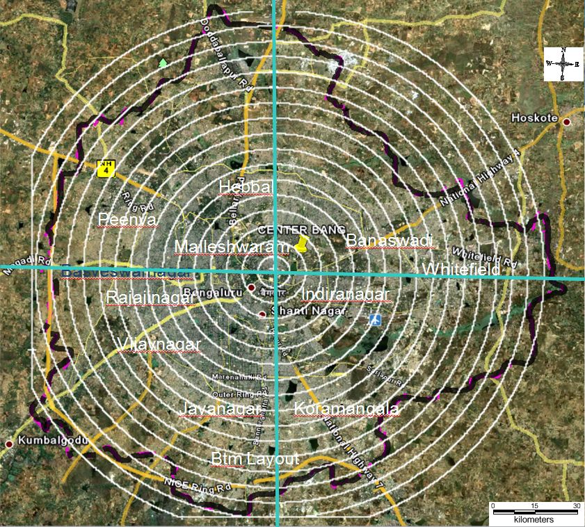
4. Density Gradient Analysis: Urbanisation pattern has not been uniform in all directions. To understand the pattern of growth vis a vis agents, the region has been divided into 4 zones based on directions - Northwest (NW), Northeast (NE), Southwest (SW) and Southeast (SE) respectively (Figure 2) based on the Central pixel (Central Business district). The growth of the urban areas in respective zones was monitored through the computation of urban density for different periods.
5. Division of these zones to concentric circles and computation of metrics: Further each zone was divided into concentric circle of incrementing radius of 1 km radius from the centre of the city (Figure 2), that would help in visualizing and understanding the agents responsible for changes at local level. These regions are comparable to the administrative wards ranging from 67 to 1935 hectares. This helps in identifying the causal factors and locations experiencing various levels (sprawl, compact growth, etc.) of urbanization in response to the economic, social and political forces. This approach (zones, concentric circles) also helps in visualizing the forms of urban sprawl (low density, ribbon, leaf-frog development). The built up density in each circle is monitored overtime using time series analysis.
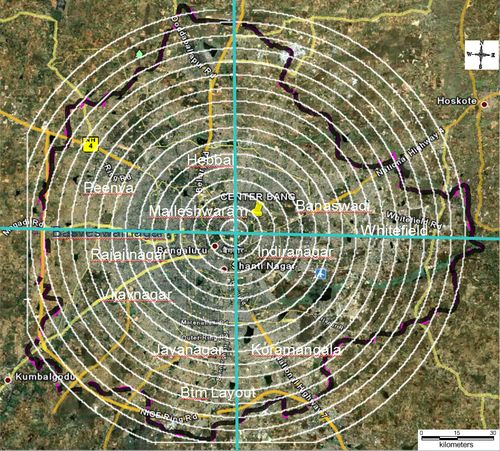
Figure 2: Division of the study area into concentric circles of incrementing radius of 1km. (Source: Google earth)
6. Computation of Shannon’s Entropy: To determine whether the growth of urban areas was compact or divergent the Shannon’s entropy (Yeh and Liu, 2001; Li and Yeh, 2004; Lata et al., 2001; Sudhira et al., 2004; Pathan et al., 2004) was computed for each zones. Shannon's entropy (Hn) given in equation 1, provides the degree of spatial concentration or dispersion of geographical variables among ‘n’ concentric circles across Zones.
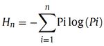 (1) (1)
Where Pi is the proportion of the built-up in the ith concentric circle. As per Shannon’s Entropy, if the distribution is maximally concentrated in one circle the lowest value zero will be obtained. Conversely, if it is an even distribution among the concentric circles will be given maximum of log n.
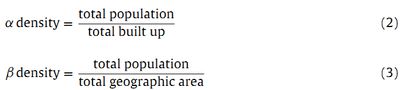
7. Computation of Alpha and Beta population density: Alpha and Beta population densities were calculated for each circle with respect to zones. Alpha population density is the ratio of total population in a region to the total builtup area, while Beta population density is the ratio of total population to the total geographical area. These metrics have been often used as the indicators of urbanization and urban sprawl and are given by:
8. Gradient Analysis of NDVI images of 1973 and 2010: The NDVI gradient was generated to visualize the vegetation cover changes in the specific pockets of the study area.
9. Calculation of Landscape Metrics: Landscape metrics provide quantitative description of the composition and configuration of urban landscape. 21 spatial metrics chosen based on complexity, centrality and density criteria (Huang et al., 2007) to characterize urban dynamics, were computed zone-wise for each circle using classified land use data at the landscape level with the help of FRAGSTATS (McGarigal and Marks, 1995). The metrics include the patch area (Built up (Total Land Area), Percentage of Landscape (PLAND), Largest Patch Index (Percentage of landscape), Number of Urban Patches, Patch density, Perimeter-Area Fractal Dimension (PAFRAC), Landscape Division Index (DIVISION)), edge/border (Edge density, Area weighted mean patch fractal dimension (AWMPFD), Perimeter Area Weighted Mean Ratio (PARA_AM), Mean Patch Fractal Dimension (MPFD), Total Edge (TE), shape (NLSI (Normalized Landscape Shape Index), Landscape Shape Index (LSI), ), epoch/contagion/dispersion (Clumpiness, Percentage of Like Adjacencies (PLADJ), Total Core Area (TCA), ENND coefficient of variation, Aggregation index, Interspersion and Juxtaposition). These metrics were computed for each region and Principal Component Analysis was done to prioritise metrics for further detailed analysis.
10. Principal Component Analysis: Principal component analysis (PCA) is a multivariate statistical analysis that aids in identifying the patterns of the data while reducing multiple dimensions. PCA through Eigen analysis transforms a number of (possibly) correlated variables into a (smaller) number of uncorrelated variables called principal components. The first principal component accounts for as much of the variability in the data as possible, and each succeeding component accounts for as much of the remaining variability as possible (Wang. 2009). PCA helped in prioritizing eight landscape metrics based on the relative contributions of each metrics in the principal components with maximum variability (Table 2).
Table 2. Prioritised landscape metrics
| |
Indicators |
Type of metrics and Formula |
Range |
Significance/ Description |
| 1 |
Number of Urban Patches |
Patch Metrics
NP equals the number of patches in the landscape. |
NPU>0, without limit. |
Higher the value more the fragmentation |
| 2 |
Perimeter Area Weighted Mean Ratio. PARA_AM |
Edge metrics
PARA _AM= Pij/Aij
Pij = perimeter of patch ij
Aij= area weighted mean of patch ij
 |
≥0, without limit |
PARA AM is a measure of the amount of 'edge' for a landscape or class. PARA AM value increases with increasing patch shape complexity. |
| 3 |
Landscape Shape Index (LSI) |
Shape Metrics
ei = total length of edge (or perimeter) of class i in terms of number of cell surfaces; includes all landscape boundary and background edge segments involving class i.
min ei = minimum total length of edge (or perimeter) of class i in terms of number of cell surfaces (see below). |
LSI>1, Without Limit |
LSI = 1 when the landscape is a single square or maximally compact patch; LSI increases without limit as the patch type becomes more disaggregated |
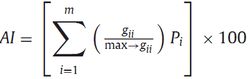
| 4. |
Clumpiness |
Compactness/ contagion / dispersion metrics
gii =number of like adjacencies (joins) between pixels of patch type (class) I based on the double-count method.
gik =number of adjacencies (joins) between pixels of patch types (classes) i and k based on the double-count method. min-ei =minimum perimeter (in number of cell surfaces) of patch type (class)i for a maximally clumped class.
Pi =proportion of the landscape occupied by patch type (class) i. |
-1≤ CLUMPY ≤1. |
It equals 0 when the patches are distributed randomly, and approaches 1 when the patch type is maximally aggregated |
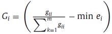
| 5. |
Aggregation index |
Compactness/ contagion / dispersion metrics
gii =number of like adjacencies (joins) between pixels of patch type (class) i based on the single count method.
max-gii = maximum number of like adjacencies (joins) between pixels of patch type class i based on single count method.
Pi= proportion of landscape comprised of patch type (class) i. |
1≤AI≤100 |
AI equals 1 when the patches are maximally disaggregated and equals 100 when the patches are maximally aggregated into a single compact patch. |
| 6. |
Interspersion and Juxtaposition |
Compactness/ contagion / dispersion metrics
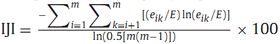
eik = total length (m) of edge in landscape between patch types (classes) i and k.
E = total length (m) of edge in landscape, excluding background
m = number of patch types (classes) present in the landscape, including the landscape border, if present. |
0≤ IJI ≤100 |
IJI is used to measure patch adjacency. IJI approach 0 when distribution of adjacencies among unique patch types becomes increasingly uneven; is equal to 100 when all patch types are equally adjacent to all other patch types. |
|