METHODOLOGY

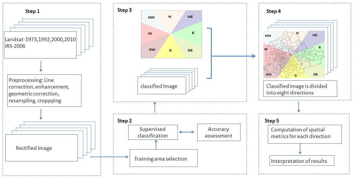
Maximum Likelihood classifier (MLC) was used to classify temporal RS data into four land use classes – builtup (urban, concrete roofs, roads, flyovers, pavements), vegetation (parks, gardens), water  bodies (lakes, ponds, wetlands) and open area (play grounds, walk ways, etc.) using the signatures generated with the training data obtained from field visits and Google Earth image. MLC is a parametric classifier that can train quickly with a capability to handle huge datasets. In fact, this also aids as ‘benchmark’ for evaluating the performance of novel classification algorithms. This method constitutes a historically dominant approach to RS-based automated LC derivation (Gao, J., 2004) and has become popular and widespread in RS because of its robustness (Hester et al., 2008). In the absence of historical data, training pixels were collected from the false colour composite of the respective bands (for the year 1973, 1992 and 2000). Since the focus of this study was to analyse the temporal urban growth pattern, so LC categories were grouped into ‘urban’ and ‘non-urban’ classes. Further, the classified images were segmented based on 8 cardinal directions. 12 spatial metrics (table 1) were computed using r.li program in GRASS (http://wgbis.ces.iisc.ernet.in/foss) and FRAGSTATS (McGarigal, 1995). The overall procedure is as depicted in figure 2.

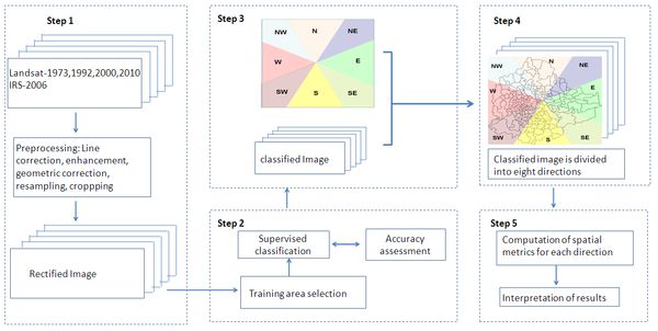
Figure 2: Schematic representation of the methods used in this study

Table 1: Description of metrics used in this study

Sl No.	Indicators	Formula	Description
1.	Largest Patch	Largest patch indicates the largest urban patch in terms of area considered	Largest urban patch in the landscape (in ha).
2.	Largest Patch Index ( Percentage of built up)	ai : area (m2) of patch i   A: total landscape area Largest Patch Index (Percentage of built up) equals the percentage of built up and landscape comprised by the largest patch respectively.	0 ≤ LPI ≤ 100. LPI = 0 when largest patch of the patch type becomes increasingly smaller. LPI = 100 when the entire landscape consists of a single patch of, when the largest patch comprise 100% of the landscape.
3.	Number of Urban Patches	NP equals the number of patches in the landscape. This is a simple measure of the extent of subdivision or fragmentation of the patch type.	NPU>0,without limit. It is a fragmentation Index
4.	Patch area distribution coefficient of variation (PADCV)	with: SD: standard deviation of patch area size Where MPS: mean patch area size, ai: area of patch i, Npatch: number of patch Patch size coefficient of variance (PADCV) is the variability in patch size relative to mean patch size. Mean Shape Index (coefficient of variation) gives the variation in the mean shape of a patch.	PADCV≥0 PADCV is zero when all patches in the landscape are the same size or there is only one patch (no variability in patch size).
5.	Mean Shape index (coefficient of variation)	Pij is the perimeter of patch i of type j. aij is the area of patch i of type j. ni is the total number of patches.	MSI ≥ 1, without limit MSI = 1 when all  patches of the corresponding patch type are circular or square; MSI increases without limit as the patch shapes becomes more irregular.
6.	Area weighted Perimeter Area Ratio	Pij: perimeter (m) of Patch ij. aij: area(m2) f patch ij. Area weighted Perimeter-Area Ratio is a simple measure of shape complexity but it varies with the size of the patch.	PARA>0, without limit
7.	Mean Patch Fractal Dimension (MPFD) coefficient of variation (COV)	Where CV (coefficient of variation) equals the standard deviation divided by the mean, multiplied by 100 to convert to a percentage, for the corresponding patch metrics. MPFD-CV indicates the variability in the complexity of urban structure expressed in percentage.	It is represented in percentage.
8.	Compactness Index (CI)	si and pi are the area and perimeter of patch i Pi  is the perimeter of a circle with the  area si N is the total number of patches. The compactness index (CI) measures not only the individual patch shape but also the fragmentation of the overall urban landscape (Huang et al., 2007). The more irregular the patch shape and patch number, the bigger the CI value.	CI value more increases with regularity of patch shape and when patch number decreases.
9.	ENND coefficient of variation	Where CV (coefficient of variation) equals the standard deviation divided by the mean, multiplied by 100 to convert to a percentage, for the corresponding patch metrics. ENND-CV represents higher variation in mean Euclidean mean nearest neighbor distance.	It is represented in percentage.
10.	Interspersion and Juxtaposition	eik: total length (m) of edge in landscape between patch types (classes) i and k. E: total length (m) of edge in landscape, excluding background m: number of patch types (classes) present in the landscape, including the landscape border, if present. Interspersion and Juxtaposition Index (IJI) equals minus the sum of the length of each unique edge type divided by the total landscape edge, multiplied by the logarithm of the same quantity, summed over each unique edge type; divided by the logarithm of the number of patch types times the number of patch types minus 1 divided by 2; multiplied by 100 to convert it to percentage.	0≤ IJI ≤100 Interspersion and Juxtaposition  approaches 0 when the distribution of adjacencies among unique patch types becomes increasingly uneven. IJI is equal to 100 when all the patch types are equally adjacent to all other patch types.
11.	Ratio of open space (ROS)	Where s is the summarization area of all “holes” inside the extracted urban area, s is summarization area of all patches Ratio of open space measures the open space compared against total urban area. Open space is crucial both as an amenity for residents and sustainability of cities.	It is represented as percentage.
12.	Patch dominance	m: number of different patch type i: patch type pi: proportion of the landscape occupied by patch type iDominance diversity index gives information if there is one dominant class in the image or if all classes have more or less same relative class proportion (Gasper and Menz, 1999).	-