|
METHODOLOGY
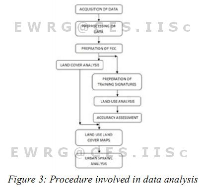
Temporal landscape dynamics are assessed through LULC changes. Figure 3 outlines the process followed for the study. Data acquisition includes obtaining data about the region such as the satellite images, Statistics, the ancillary data (Gazetteer, Census), the Maps such as Village maps, District maps. Preprocessing of the data is done to remove the haze and other factors through atmospheric correction, removal of noise and other radiometric errors through radiometric corrections. Image enhancement is done using standard image processing techniques. The data pertaining to the studyregion is extracted by cropping using the boundary. For visual interpretation and for creation of the training sets for classification of the images, a false color Composite (FCC) image of the study area is created. FCC is created by composition of band2 (green), band3 (red) and band4 (IR).
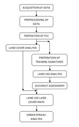
Figure 3: Procedure involved in data analysis
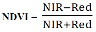
Assessment of landscape dynamics involves the analysis of temporal land use and land cover. Land cover analysis involves the computation of extent of vegetation through well-established vegetation indices. Vegetation indices help in mapping the regions under vegetation and non-vegetation. Vegetation Indices are the Optical measures of Vegetation Canopy. Vegetation indices are dimensionless radiometric measurements that indicate the relative abundance and activity of green vegetation; this includes the leaf area index (LAI), percentage green cover, chlorophyll content, and green biomass. The main requirement of vegetation indices measurement is to combine the chlorophyll absorbing (Red Band) spectral region with the non-absorbing (NIR band) spectral region to provide a consistent and robust measure of area under the canopy. Vegetation Indices algorithms are designed to extract the active greenness signal from the terrestrial land cover. The accuracy of the VI product varies with time, space, geology, seasonal variations, canopy background (soil, water).Among all techniques Normalized Difference Vegetation Index (NDVI) is most widely used for LC analysis. NDVI is expressed as the ratio of difference in NIR and Red bands to the sum of NIR and Red band. NDVI has the ability to minimize the topographic effect in the region. NDVI ranges between -1 to +1, ratio less than 0 i.e., the negative values represent non-vegetation and positive values represent vegetation.
Land use analysis involves categorizing each pixel in the spatial data into different land use themes such as water bodies, vegetation, built up, cultivable land, barren lands, etc.A multispectral data is useful to perform classification as it shows the numerous spectral patterns/signatures for different features. Spectral pattern recognition refers to the family of classification procedures that utilizes pixel by pixel spectral information as a basis for land use classification. Land use analysis involves collection of training data from field, attribute data for the chosen polygons in FCC, and goggle earth. These training sets were employed for classification of the data into various classes. 60% of training data is used from classifying the spatial data, while the balance has been used for verification. GRASS GIS, open source software was used for analysis of the data. Land use analysis was carried out using the Gaussian maximum likelihood classifier (GMLC) algorithm.Accuracy assessment is done through error matrix, comparing on a category by category basis, the relationship between reference data (ground truth) and the corresponding classified results.
Computation of Shannon’s entropy: Shannon’s entropy (Yeh and Li, 2001, Ramachandra et al., 2012) was computed to detect the urban sprawl phenomenon and is given by,
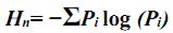
Where; Pi is the Proportion of the urban density in the ith zone and n the total number of zones. This value ranges from 0 to log n, indicating very compact distribution for values closer to 0. The values closer to log n indicates that the distribution is much dispersed. Larger value of entropy reveals the occurrence of urban sprawl.
|