
Data and method
1. Remote sensing (RS) data
The RS data used in the study include Landsat MSS (1973), TM (1989, 2000), Landsat ETM+ (2003, 2004), IRS LISS-IV MX (2009, 2010), and Google Earth (http://earth.google.com). The Landsat data is cost effective, with high spatial resolution and freely downloadable from public domains like GLCF (http://glcfapp.glcf.umd.edu:8080/esdi/index.jsp) and USGS (http://glovis.usgs.gov/). The different seasonal data (summer, post monsoon) is considered to account the adverse effect of seasonal variation in canopy light interception. The summery characteristics of datasets used in the current study are summarized in Table 1.
Table 1. Details of remote sensing data
| Year | Satellite | Date of Acquisition | Resolution (m) |
| 1973 | Landsat MSS | 02/11/1973 | 57 |
| 1989 | Landsat TM | 19/11/1989 | 28.5 |
| 2000 | Landsat TM | 25/11/2000 | 30 |
| 2003 | Landsat TM | 01/02/2003 | 30 |
| 2004 | Landsat ETM+ | 22/11/2004 | 30 |
| 2010 | IRS P6 L4 MX | – | 5 |
2. Ancillary data
Ancillary data provides helpful information to assist the interpretation of different land use types from remotely sensed images. Besides remote sensing data, many other data sources were used in the study. The multi-data areused to make use of different data sets available for better interpretation and to improve the accuracy of the datasets. Frequently used ancillary data are the Survey of India topographic maps at varying scales (1:50000, 1:250000). Topographic maps provided ground control points to rectify remotely sensed images and scanned historical paper maps. The population data (2001, 2011 census) collected from the directorate of census operation is used to analyse the population distribution of study area. Other ancillary data includes land cover maps, administration boundary details, transportation data (road network) and field data using GPS(Global Positioning System – Garmin GPS).
3. Method
Figure 2 illustrates the method adopted for the analysis. RS data of different sensors of Landsat (a series of earth resource scanning satellites launched by the USA) were downloaded from the public domain (http://glovis.usgs.gov) while IRS (Indian Remote Sensing Satellites) data were procured from the National Remote Sensing Centre, Hyderabad (http://www.nrsc.gov.in). These data were preprocessed for atmospheric and geometric corrections to enable correct area measurements, precise localization and multi-source data integration (Jixian etal.2007). The field investigation is carried out for the collection of ground control points (GCP’s) and training data (with attribute data) studies during pre-monsoon and post-monsoon seasons. The geographic coordinates of a land cover classes (of the training polygons) are determined by using pre-calibrated GARMIN GPS – Global Position Systems. Historical land-cover data were compiled from the forest department records apart from the interviews and group discussions with the local farmers and forest officials. Geometric correction is implemented by using ground control points collected from field using GPS. Landsat data is resampled to 30 meters, for comparison across multi-resolution data of Landsat sensors with dissimilar spatial resolutions.
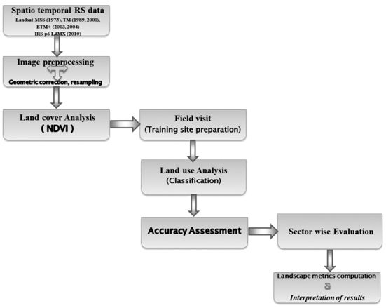
Fig. 2. Method for spatio temporal analysis using remote sensing data
NDVI (Normalized Difference Vegetation Index) was computed with the temporal data for land cover analysis. NDVI is based on the principle of spectral difference based on strong vegetation absorbance in the red and strong reflectance in the near-infrared part of the spectrum. Vegetation index differencing technique was used to analyse the amount of change in vegetation (green) versus non-vegetation (non- green) with the two temporal data of 1973 and 1989 as reference. Calculation of NDVI for Multi-temporal data is advantageous in areas with rapid vegetation changes. Among numerous vegetation indices for land cover mapping, NDVI is most widely accepted and applied (Ramachandra et al. 2009). NDVI is calculated using visible Red (0.63–0.69 μm) and NIR (0.76–0.90 μm) bands of Landsat TM/ETM+. NDVI for a given pixel ranges from minus one (–1) to plus one (+1). NDVI was calculated using Eq. (1):
The land use analysis was done using supervised classification scheme with selected training sites. Image classification pursues to categorize features on the image based on their spectral character. Gaussian Maximum Likelihood classifier (GMLC) is a common, appropriate and efficient method in supervised classification techniques by using multi-temporal “ground truth” information with the suitable training set for classifier learning.
Supervised training areas are located in regions of homogeneous land use classes: built-up, water, cropland, grass lands (degraded forest), open space or barren land, deciduous forest, evergreen forest. GRASS GIS (Geographical Analysis Support System, http://ces.iisc.ac.in/grass) a free and open source software having the robust support for processing both vector and raster files is used for LULC analysis. An accuracy assessment is done to assess the quality of the information derived from remotely sensed data by a set of reference pixels. These test samples are then used to generate the error matrix (also referred as confusion matrix) kappa (κ) statistics and producer’s (PA) and user’s accuracies (UA) to assess the classification accuracies. Kappais an accuracy statistic that permits us to compare two or more matrices andweighs cells in error matrix according to the magnitude of misclassification. Accuracy assessment with kappa statistics has been done, which aided in evaluating the strength of each class as well as the efficacy of classification technique.
In order to access the detailed LULC pattern, a study is carried out at macro and micro scales by considering the whole landscape as a single unit and sector based analysis. The study area has been divided in to 12 sectors/segments as the landscape is of varying topography with diverse land use; each sector covers around 13km length as shown in Figure 3. Landscape dynamics was analysed for each sector for 1973, 1989, and 2010 through landscape metrics using FRAGSTAT 3.3 (McGarigal et al. 2002) to explain the spatial heterogeneity changes in the region. A set of significant indicators were prioritized for a detailed analysis of the landscape. Table 2 lists the chosen metrics with range and descriptions. In the regional planning, demographic aspect is one of the most significant aspects as decentralized planning would be effective. The population density is computed to understand the spatial dimensions in human settlements. Density gradient metrics computation is done using Alpha and Beta population density to investigate land transformation with respect to population in each sector. Alpha population density is the ratio of total population in a region to the total built-up area, while Beta population density is the ratio of total population to the total geographical area. These metrics have been often used as the indicators of urbanization and urban spread (Sudhira et al. 2004; Ramachandra et al. 2012) and are given by:
 ................... (2)
 .............(3)
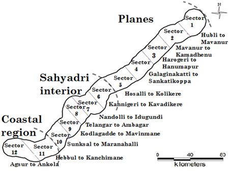
Fig. 3. Sector based divisions of study area
Table 2. Landscape metrics selected in the study
| Indicators | Formula | Range | Significance | |
| 1 | Number of Urban Patches | NP equals the number of patches in the landscape. | NPU>0, without limit. | Higher the value more the fragmentation. |
| 2 | Largest Patch Index (Percentage of built up) | a i = area (m2) of patch i; A= total landscape area. |
0 ≤ LPI ≤ 100 | LPI = 0 when largest patch of the patch type becomes increasingly smaller. LPI = 100 when the entire landscape consists of a single patch |
| 3 | Perimeter Area Weighted Mean Ratio. PARA_AM | Pij = perimeter of patch ij; Aij= area weighted mean of patch ij. |
> 0,without limit | PARA AM is a very useful measure of fragmentation; it is a measure of the amount of ‘edge’ for a landscape or class. PARA AM value increased with increasing patch shape complexity, which characterize the degree of patch shape complexity. |
| 4 | Area Weighted Mean Shape Index (AWMSI) | Where Si and Piare the area and perimeter of patch i, and N is the total number of patches. | AWMSI ≥ 1, without limit | AWMSI = 0 when all patches in the landscape are circular or square. AWMSI increases without limit as the patch shape becomes irregular. This index represents the shape irregularity of patches. The higher this value is, the more irregular the shapes are. |
| 5 | Area weighted Euclidean mean nearest neighbor distance ENN_AM | hijisdistance (m) from patch ij to nearest neighboring patch of the same type(class) based on shortest edge to edge distance. | ENN>0, without limit | ENN approaches zero as the distance to the nearest neighbor decreases. ENN_AM is used to calculate relative distance between the patches of same class. |
| 6 | Shannon’s diversity index | i – patch type; m – number of patch type; pi – proportion of the landscape occupied by patch type i. |
Range: SHDI ≥ 0, without limit | Shannon’s diversity index is a measure of diversity. SHDI increases as the number of different patch types (patch richness, PR) increases or the proportional distribution of area among patch types becomes more equitable, or both. |
Prediction of likely changes has been done through scenario analysis, using LULC change as an input. The model generated possible scenarios of land-use changes considering the current rate of LU changes and also by considering the likely developmental projects, along with various indicators like deforestation and fragmentation. The spatial dynamic models have become an inseparable aspect of a planning system in this regard, model has been implemented using NetLogo (Wilensky 1999), an agent-based modelling environment developed by the Centre for Connected Learning and Computer Based Modeling, Northwestern University, USA, which facilitates encapsulation of processes through rule-based procedures and offers adequate monitors and plots to visualise pattern, model the causes and evaluate the consequences through simulation.