|
RESULTS
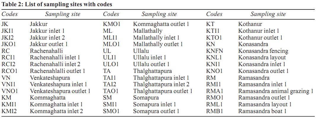
Water quality analysis
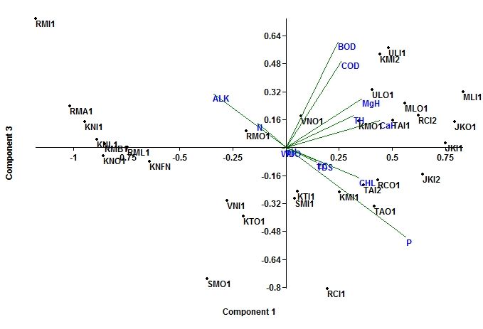
Table 3 lists the physical and chemical parameters, which indicate significant variations across wetlands. pH, EC, BOD and COD values indicated marked difference among as well as within wetlands. pH was lowest at Jakkur (JK) outlet (7.89), highest at Mallathally (ML) inlet (10.30) and beyond the permissible limits at Kommaghatta (KM), Kothanur (KT) and Rachenahalli (RC) sites. JK (1267.44µScm-1) comprised high electric conductivity followed by Somapura (SM) (1022.67µScm-1) and the least EC was observed at Venkateshpura (VN, 351.75 µScm-1) followed by Ramasandra (RM, 494.4 µScm-1). Sampling sites such as RC, VN, KM, RM and SM reflected low organic matter in terms of BOD whereas high at JK, ML, Thalghattapura (TH), Ullau (UL), Kothanur (KT) and Konasandra (KN). The consistent high organic pollution in terms of COD was recorded at all wetlands with exception at few sites such as RCI1, KMI1, SMO1, KNO1, RMA1 and RMB1 (refer table 2 for codes and respective sampling sites). Nitrates and phosphates were within the permissible limits ranging between 0.015 to 0.092 mgL-1 and 0.001 to 0.064 mgL-1 respectively. Total hardness ranged between 67.5 mgL-1 (KTO1) to 346.67 mgL-1 (JKI2) and increased at MLO1 and JKI1. Chlorides level reflected impacts on KNI1 (41.75 mgL-1), JK, RCI2, MLI1 and JKI2 (295.36 mgL-1) where inflow of sewage and urbanization was intensely noticed. PCA biplot (Figure 3) explains 44.799% and 12.453 % variance from 1st and 3rd components respectively, and separates most polluted sites from least polluted sites. The PC1 explained influence of P at RC, KTI1, TAO1 and KMI1 sites. EC, TH, CaH, MgH and CHL were significantly high at right side of PC1 influencing ML, UL, JK and TH inlet sites where inflow of sewage with high ionic concentrations was apparent. The high alkalinity was evident through PC3 at RM and KN sites.
Table 3. Variation in water physical and chemical analysis across lakes.
(Sampling codes are mentioned in Table 2)
Sampling
Site |
pH |
WT oC |
EC
µScm-1 |
TDS
mgL-1 |
DO
mgL-1 |
BOD
mgL-1 |
COD
mgL-1 |
N
mgL-1 |
P
mgL-1 |
TH
mgL-1 |
CaH
mgL-1 |
MgH
mgL-1 |
CHL
mgL-1 |
ALK
mgL-1 |
| JKI1 |
8.02 |
27.8 |
1240.33 |
870.67 |
4.67 |
14.2 |
79.31 |
0.016 |
0.026 |
326.67 |
193.33 |
56.93 |
286.84 |
163.33 |
| JKI2 |
8.07 |
28.77 |
1325.67 |
947 |
6.91 |
13.6 |
48.72 |
0.015 |
0.03 |
346.67 |
100 |
60.19 |
295.36 |
163.33 |
| JKO1 |
7.89 |
28.6 |
1236.33 |
869.33 |
4.76 |
8.2 |
65.08 |
0.016 |
0.027 |
325.33 |
185.33 |
58.56 |
267.91 |
160 |
| RCI1 |
9.22 |
30.33 |
871.33 |
625 |
6.12 |
2.9 |
11.71 |
0.018 |
0.026 |
221.33 |
184.67 |
33.35 |
195.96 |
126.67 |
| RCI2 |
9.1 |
30.07 |
885.67 |
620 |
7.75 |
4.05 |
77.55 |
0.018 |
0.023 |
221.33 |
172.67 |
36.27 |
208.27 |
120 |
| RCO1 |
9.05 |
31.33 |
854.33 |
609.33 |
7.32 |
3.22 |
35.91 |
0.02 |
0.023 |
222.67 |
180 |
34.81 |
191.23 |
120 |
| VNI1 |
8.54 |
28.15 |
342 |
239 |
8.13 |
3.11 |
26.88 |
0.02 |
0.022 |
122 |
63.33 |
14.31 |
45.44 |
100 |
| VNO1 |
8.21 |
24.95 |
361.5 |
247.5 |
6.18 |
5.22 |
83.45 |
0.02 |
0.027 |
152 |
56 |
23.42 |
44.02 |
95 |
| KMI1 |
9.32 |
28.05 |
812 |
594 |
5.98 |
2.96 |
24 |
0.049 |
0.038 |
264 |
124.05 |
58.55 |
121.41 |
276 |
| KMI2 |
9.01 |
29.05 |
782 |
558 |
4.55 |
5.3 |
84 |
0.056 |
0.02 |
298 |
150.23 |
69 |
109.48 |
248 |
| KMO1 |
8.98 |
28.7 |
764.5 |
548.5 |
6.14 |
3.71 |
48 |
0.066 |
0.022 |
286 |
132.87 |
61.76 |
119.42 |
170 |
| MLI1 |
10.3 |
26.65 |
1160 |
807 |
9.39 |
25.8 |
110 |
0.072 |
0.064 |
278 |
132.87 |
59.81 |
214.42 |
252 |
| MLO1 |
9.28 |
31.45 |
1105 |
803 |
7.44 |
18 |
69 |
0.062 |
0.046 |
302 |
124.05 |
67.82 |
106.5 |
301 |
| ULI1 |
8.8 |
28.75 |
747.5 |
514 |
7.03 |
6.5 |
106 |
0.092 |
0.037 |
298 |
123.25 |
67.04 |
80.94 |
315 |
| ULO1 |
8.97 |
26.05 |
587 |
416.5 |
6.59 |
4.91 |
82 |
0.078 |
0.041 |
224 |
120.04 |
49.77 |
80.94 |
210 |
| TAI1 |
8.98 |
30.1 |
779 |
536 |
11.54 |
14.35 |
70 |
0.048 |
0.045 |
178 |
136.87 |
34.43 |
185.31 |
252 |
| TAI2 |
8.92 |
29.2 |
788.5 |
548 |
11.18 |
13.26 |
34 |
0.058 |
0.054 |
190 |
129.66 |
39.12 |
187.44 |
293 |
| TAO1 |
8.45 |
29.55 |
790.5 |
670 |
5.61 |
2.67 |
30 |
0.043 |
0.049 |
180 |
136.87 |
34.92 |
184.6 |
163 |
| SMI1 |
8.77 |
29.47 |
1020.67 |
708.67 |
6.69 |
2.88 |
36 |
0.078 |
0.044 |
112.67 |
81 |
19.93 |
120.7 |
265.33 |
| SMO1 |
8.72 |
30.2 |
1024.67 |
709.67 |
6.29 |
2.31 |
26.67 |
0.075 |
0.046 |
109.33 |
33.67 |
18.46 |
82.36 |
286.67 |
| KTI1 |
9.13 |
30.05 |
681 |
472 |
6.91 |
20.58 |
31 |
0.068 |
0.056 |
82.5 |
55.05 |
14.02 |
142 |
194 |
| KTO1 |
9.12 |
29.15 |
653 |
467 |
7.56 |
23.5 |
12 |
0.079 |
0.056 |
67.5 |
23.05 |
10.85 |
139.16 |
192 |
| KNFN |
8.8 |
33.43 |
792 |
551.33 |
6.37 |
2.63 |
38.67 |
0.067 |
0.015 |
88.67 |
22.98 |
16.03 |
69.2 |
406 |
| KNL1 |
8.8 |
31.47 |
718 |
548 |
6.41 |
2.35 |
30.67 |
0.067 |
0.006 |
86 |
22.98 |
15.38 |
57.46 |
334.67 |
| KNI1 |
8.97 |
32.43 |
766 |
537.67 |
7.28 |
13.44 |
49.33 |
0.058 |
0.005 |
80 |
23.99 |
13.67 |
41.75 |
327.33 |
| KNO1 |
8.69 |
31.67 |
825.67 |
582 |
6.11 |
13.75 |
26.67 |
0.07 |
0.007 |
85.33 |
24.9 |
14.74 |
71.95 |
398 |
| RMI1 |
8.85 |
31 |
490 |
343 |
6.67 |
2.88 |
44.89 |
0.051 |
0.001 |
113.33 |
80.73 |
20.16 |
59.92 |
1088.67 |
| RMA1 |
8.96 |
31.1 |
466 |
369.33 |
6.05 |
1.92 |
19.11 |
0.067 |
0.004 |
129.33 |
33.13 |
23.47 |
61.53 |
788.67 |
| RMO1 |
8.6 |
31.1 |
496 |
356 |
7.06 |
3.33 |
58.67 |
0.039 |
0.02 |
164 |
121.28 |
29.94 |
100.82 |
744 |
| RML1 |
8.88 |
28.97 |
516.67 |
357.67 |
6.21 |
2.68 |
36.44 |
0.047 |
0.014 |
112.67 |
34.2 |
19.15 |
65.13 |
974 |
| RMB1 |
8.86 |
30.07 |
503.33 |
353.67 |
6.37 |
4.59 |
17.79 |
0.027 |
0.006 |
107.33 |
93.67 |
17.97 |
64.94 |
1100.67 |
| PL * (BIS) |
6.5-9 |
-- |
<1200 |
<500 |
>5 |
<3 |
<30 |
<45 |
-- |
<300 |
<80 |
-- |
<200 |
<600 |
*Permissible limits
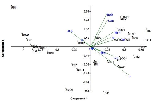
Fig 3. PCA bi-plot showing water physico chemical variation across sampling sites.
(Sampling codes are mentioned in Table 2)
Species richness, diversity and distribution
40 diatom genera comprising 91 species were found on 33 sampled habitats, with 10 species occurring at ≥10% relative abundances in at least one sample (Annexure I). The most common and abundant species were Achnanthidium Kützing, Cyclotella meneghiniana Kützing, Diadesmis confervaceae Kützing, Gomphonema Ehrenberg, Nitzschia palea (Kutzing) W. Smith, Amphora veneta Kützing, Gyrosigma rautenbachiae Cholnoky and Cymbella kappi (Cholnoky) Cholnoky, The species belonging to genera Achnanthidium was not further identified due to complexity in the species and its wide range of occurrence. Two Gomphonema sp. could not be identified to species level. More number of taxa (24) was recorded at UL and lowest at VN (9.50).
A total of 16 macroinvertebrates samples were identified from 27 sites up to family level and 2 till order level. The macroinvertebrates were represented by 19 families of aquatic insects, among them, the dominant were Belostomatidae, Corixidae, Diptera, Gerridae, Damsel fly, Odonata, and Pleidae and, 8 Mollusca family such as Viviparidae, Lymnaeidae, Physidae, Planorbidae and Thiaridae were dominant (Annexure II and III). The contribution of the most common and abundant families to the total of macroinvertebrates were Corixidae (22.69 %; JKO1 and 44.27 %; MLI), Nepidae (7.80%; JKI1), Notonectidae (58.40%; JKO1), Physidae (37.16; MLI1) and Planorbidae (9.87%; MLI1). Family Corixidae and Physidae at site MLI1 showed highest abundance of 305 and 256 respectively. The species such as Lamellidens consobrinus, Physa acuta, Segmentina (Polypylis) taia, and Thiara (Thiara) scabra, and genus Gabbia, Pisidium and Tarebia are first time recorded from this region.
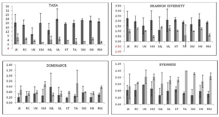
The diatom and macroinvertebrate assemblage were compared for its dominance, evenness and species richness (Figure 4). Shannon diversity index for diatoms was highest at JK (2.27) and lowest at ML (1.10), while macroinvertebrate diversity index was highest at ML (1.40) and lowest was recorded as 0.49 at KM. Dominance ranged between 0.18 to 0.58 (diatoms) and 0.30 to 0.72 (macroinvertebrates). ML (0.58) had highest diatom dominance of C. meneghiniana whereas macroinvertebrate species Physa acuta was highest dominant at TH. None of the sampling sites except VN (0.58) had evenness index more than 50%. VN being the least polluted site with low ionic concentrations, inhabit pollution sensitive species such as Achnanthidium sp., and Cymbella sp. Evenness ranged from 0.54 (JK) to 1 (TH), and the distribution of macroinvertebrates was observed with the changing levels of pollution (Table 3).
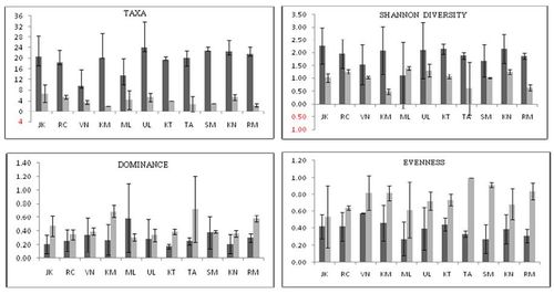
Fig 4. Bar graph showing comparison of diatoms with macroinvertebrates in number of taxa, Shannon diversity index, Dominance and Evenness index across sampling sites. Black bar represents diatoms and grey represents macroinvertebrates.
(The sampling sites and codes are mentioned in Table 2)
Relationship between water chemistry and indices
The correlation among environmental variables with the diatom and macro invertebrate indices is listed in Table 4. Among water chemistry variables, pH correlated with DO and N whereas, CHL correlated well with EC and N. BOD with P correlated significantly indicating the profuse growth of algae (algal blooms) with high P concentration leading to high BOD. The alkalinity also showed correlation with CHL and P which attributes to pollution. %PT significantly correlated with ALK and GDI index showed a significant, but negative correlation with TDI and %PT. The strong correlation was also observed, BI with EC (0.481) while FBI with N (0.424) signifying trophic status. The comparison of the indices resulted in a very good negative correlation between TDI and GDI (-0.64), %PT and GDI (-0.712) and a positive correlation between FBI and BI (0.975).
Table 4. Spearman correlation between major environmental variables and indices derived from diatoms and macroinvertebrates. (n= 27, p<0.05)
(Codes are mentioned in Table 2)
| |
pH |
EC |
DO |
BOD |
COD |
N |
P |
CHL |
ALK |
TDI |
%PT |
GDI |
BI |
FBI |
| pH |
0 |
|
|
|
|
|
|
|
|
|
|
|
|
|
| EC |
0.051 |
0 |
|
|
|
|
|
|
|
|
|
|
|
|
| DO |
0.493 |
0.113 |
0 |
|
|
|
|
|
|
|
|
|
|
|
| BOD |
0.370 |
0.352 |
0.377 |
0 |
|
|
|
|
|
|
|
|
|
|
| COD |
0.117 |
0.203 |
0.115 |
0.176 |
0 |
|
|
|
|
|
|
|
|
|
| N |
0.525 |
0.077 |
0.145 |
0.221 |
0.040 |
0 |
|
|
|
|
|
|
|
|
| P |
0.385 |
0.275 |
0.386 |
0.492 |
0.099 |
0.355 |
0 |
|
|
|
|
|
|
|
| CHL |
0.177 |
0.739 |
0.058 |
0.346 |
0.202 |
0.448 |
0.338 |
0 |
|
|
|
|
|
|
| ALK |
0.082 |
0.352 |
0.056 |
0.233 |
0.117 |
0.163 |
0.456 |
0.404 |
0 |
|
|
|
|
|
| TDI |
0.070 |
0.554 |
0.192 |
0.636 |
0.529 |
0.235 |
0.188 |
0.675 |
0.054 |
0 |
|
|
|
|
| %PT |
0.012 |
0.309 |
0.035 |
0.067 |
0.004 |
0.038 |
0.299 |
0.173 |
0.650 |
0.282 |
0 |
|
|
|
| GDI |
0.212 |
0.213 |
0.147 |
0.269 |
0.088 |
0.135 |
0.056 |
0.023 |
0.321 |
-0.640 |
-0.712 |
0 |
|
|
| BI |
0.203 |
0.481 |
0.228 |
0.234 |
0.152 |
0.366 |
0.288 |
0.191 |
0.091 |
0.159 |
0.100 |
0.292 |
0 |
|
| FBI |
0.262 |
0.246 |
0.192 |
0.256 |
0.149 |
0.424 |
0.318 |
0.139 |
0.138 |
0.106 |
0.130 |
0.324 |
0.975 |
0 |
Variation in Indices
There was not much difference found in the indices scores between TDI and GDI, and between FBI and BI. The overall dissimilarity was observed to be 14.57% and 38.6% in diatom and macroinvertebrate indices respectively. However, TDI and BI indices were used in further clustering of sites because of the accuracy and these comprise score for most of the taxa recorded in this study and have been represented as modified index table in Table 5. TDI value ranged from 0 to 20 revealing high trophic level as score increases to 20 and clean water as the score decreases. TDI with much variation ranged between 3.3- 17.28 and sites were grouped based on the classes mentioned in table 5. BI indices ranged from 0 to 10, the increasing score indicated increasing levels of pollution. BI ranged between 0-6.5 and follows 6 classes as mentioned in Table 5.
Table 5. Modified index table of Diatom (TDI) and Macroinvertebrate (BI) indices reflecting water quality and respective trophic status. (Source: Kelly et al., 1998 and Bode et al., 2002).
| SL. NO |
TDI |
TROPHY |
BI |
STATUS |
DEGREE OF ORGANIC POLLUTION |
CLASS |
| 1 |
<9 |
Oligotrophy |
0-3.5 |
Excellent |
No apparent organic pollution |
Class I |
| 2 |
9-12 |
Oligo-mesotrophy |
3.51-4.50 |
Very good |
Possible slight organic pollution |
Class II |
| 3 |
12-15 |
Mesotrophy |
4.51-5.50 |
Good |
Some organic pollution |
Class III |
| 5.51-6.5 |
Fair |
fairly significant organic pollution |
| 4 |
15-17 |
Meso-
eutrophy |
6.51-7.5 |
Fairly poor |
Significant organic pollution |
Class IV |
| 5 |
>17 |
Eutrophy |
7.51-8.5 |
Poor |
Very Significant organic pollution |
|
| 8.51-10 |
Very poor |
Severe organic pollution |
Class V |
Variation in water quality and species composition among interconnected wetlands
Data analysis reveals of a marked difference between Jakkur and Rachenahalli in terms of water quality. pH of Jakkur was ranging from 7.89-8.02 and Rachenahalli had high alkaline range (9.05-9.22). There was no difference in the nutrient load but higher values for BOD, COD, total hardness and chlorides concentration was observed at Jakkur compared to Rachenahalli. The Shannon diversity index was 2.27 and 1.03 at Jakkur and, 1.97 and 1.26 at Rachenahalli representing diatom and macroinvertebrate diversity respectively. However, there was a significant dissimilarity in species composition. The dominant diatom taxa at Jakkur were CMEN, DCOF and macroinvertebrate were Belostomatidae and Gerride groups. The dominant diatom taxa at Rachenahalli were ACHD, CMEN, FBCP and NAMP, and Lymnaeidae, Planorbidae and Diptera groups.
Clustering of wetlands
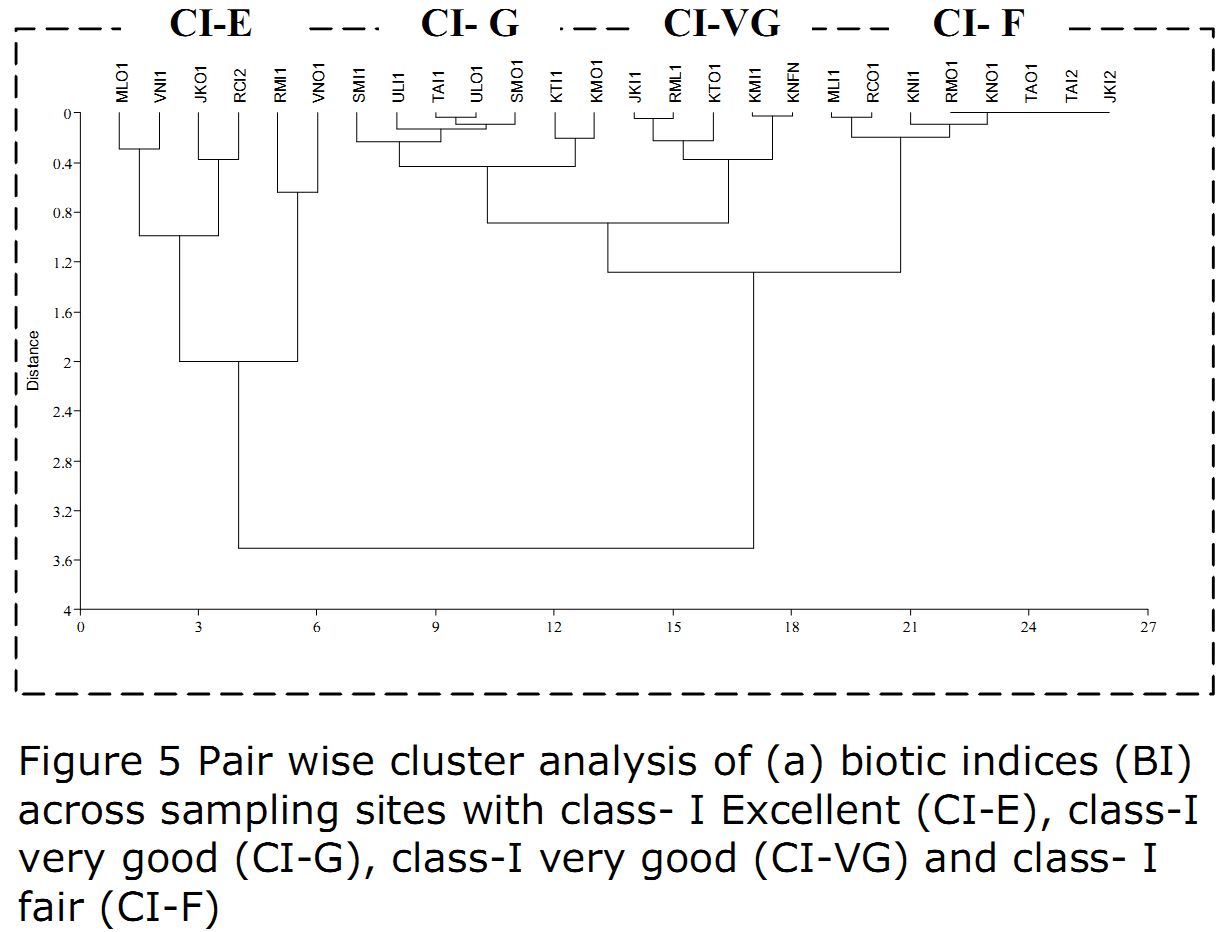
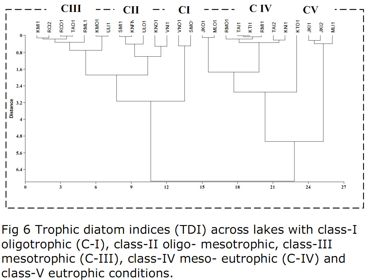
Figure 5 and Figure 6 explain the pair-wise clustering of sampling sites based on the macroinvertebrate community and diatom indices respectively and are grouped into 5 classes (Table 5). The variation in classification of sites was significant in both the indices. Macroinvertebrate index tended to have slightly lower variation in index values characteristic of lack of species data. According to TDI, 2 sampling sites were clustered under class I, SM and VN as oligotrophic status or clean water and, outlets of UL, KN and inlets of SM and VN sites with slightly higher values under class II. Class III includes sites such as TA, RM, RC, KM and ULI1 indicating oligo-mesotrophic conditions. Class IV and V mainly comprised sampling sites of JK, ML, TA and KT with heavy pollution. BI grouped 6 sites as oligotrophic and 13 sites as oligo-mesotrophic condition. Whilst the inlets of JK, KN, ML and outlets of TA, KN, RM and RC were in mesotrophic condition (C III).In the BI clustering, none of the sites were grouped under class IV and V.
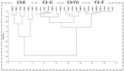
Fig 5. Pair wise cluster analysis of (a) biotic indices (BI) across sampling sites with class- I Excellent (CI-E), class-I very good (CI-G), class-I very good (CI-VG) and class- I fair (CI-F)
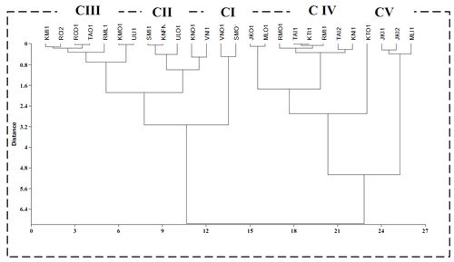
Fig 6. Trophic diatom indices (TDI) across lakes with class-I oligotrophic (C-I), class-II oligo- mesotrophic, class-III mesotrophic (C-III), class-IV meso- eutrophic (C-IV) and class-V eutrophic conditions.
|
