|
RESULTS AND DISCUSSION
Land use Land Cover analysis:
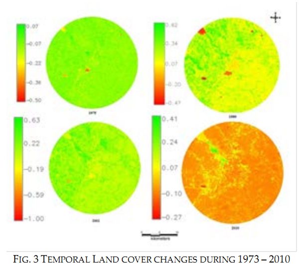
Vegetation cover analysis: Vegetation cover of the study area assessed through NDVI (Fig. 3), shows that area under vegetation has declined by about 19%. Temporal NDVI values are listed in Table III, which shows that there has been a substantial increase in the Non Vegetative area. There has been an increase from 3 % to 17%, tells us that there has been staggering growth of impervious cover in the region resulting from decrease in vegetative cover.
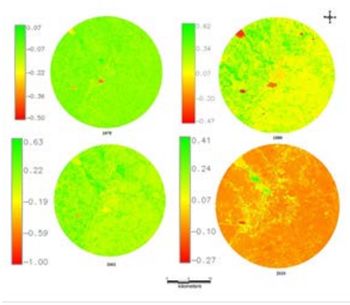
Fig. 3. Temporal Land cover changes during 1973 – 2010
Table III. Landscape metrics analysed
| |
Indicators |
Formula |
Range |
| 1 |
Number of Urban Patches (NPU) |

NP equals the number of patches in the landscape. |
NPU>0, without limit. |
| 2 |
Patch density(PD) |
f(sample area) = (Patch Number/Area) * 1000000 |
PD>0 |
| 3 |
Normalized Landscape Shape Index (NLSI) |

Where si and pi are the area and perimeter of patch i, and N is the total number of patches. |
0≤NLSI<1 |
| 4 |
Landscape Shape Index (LSI) |

ei =total length of edge (or perimeter) of class i in terms of number of cell surfaces; includes all landscape boundary and background edge segments involving class i.
Min ei=minimum total length of edge (or perimeter) of class i in terms of number of cell surfaces. |
LSI>1, Without Limit |
| 5 |
Clumpiness |
 
gii =number of like adjacencies between pixels of patch type gik =number of adjacencies between pixels of patch types i and k.
Pi =proportion of the landscape occupied by patch type (class) i. |
-1≤ CLUMPY ≤1. |
| 6 |
Percentage of Like Adjacencies (PLADJ) |
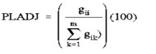
gii = number of like adjacencies (joins) between pixels of patch type gik = number of adjacencies between pixels of patch types i and k |
0<=PLADJ<=100 |
| 7 |
Aggregation index (AI) |

gii =number of like adjacencies between pixels of patch type
Pi= proportion of landscape comprised of patch type. |
1≤AI≤100 |
| 8 |
Cohesion |
 |
0≤cohesion<100 |
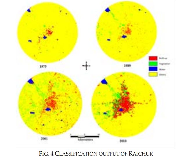
Land use analysis: Land use assessed during the period from 1973 to 2010 by means of Gaussian maximum likelihood classifier is listed in Table IV and the same is depicted in Fig. 4. The overall accuracy of the classification ranges from 69.28% (1973) to 88.12% (2010). Kappa statistics and overall accuracy was calculated and listed in Table V. There has been a significant increase in built-up area during the last decade evident from 590% increase in urban area 1.44% in 1975 and has grown to 8.51% considering buffer area. Other category also had an enormous decrease in the land use. Consequently, cultivable area has come down drastically.
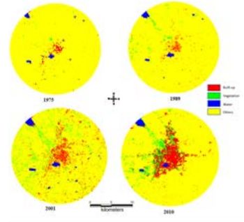
Fig. 4. Classification output of Raichur
Table IV: Temporal land use details for Raichur
| Land use |
Urban |
Vegetation |
Water |
Cultivation and others |
| Year |
| 2010 |
8.51 |
4.81 |
0.97 |
85.71 |
| 2002 |
5.21 |
3.58 |
1.36 |
89.85 |
| 1992 |
2.48 |
0.91 |
1.04 |
95.57 |
| 1973 |
1.44 |
1.62 |
0.88 |
96.16 |
Table V: Kappa statistics and overall accuracy
| Year |
Kappa coefficient |
Overall accuracy (%) |
| 1973 |
0.69 |
69.28 |
| 1989 |
0.83 |
81.69 |
| 1999 |
0.83 |
84.53 |
| 2010 |
0.89 |
88.12 |
Shannon’s entropy: The entropy is calculated considering 7 gradients in 4 directions and listed in table VI. The reference value is taken as Log (7) which is 0.77 and the computed Shannon’s entropy values are closer to this, indicating sprawl. Increasing entropy values from 1973 to 2010 shows the tendency of dispersed growth of built-up area in the city with respect to 4 directions as we move towards the outskirts and this phenomenon is most prominent in SE and SW directions.
Table VI: Shannon Entropy Index
|
NE |
NW |
SE |
SW |
| 2010 |
0.135 |
0.146 |
0.168 |
0.194 |
| 2002 |
0.078 |
0.083 |
0.084 |
0.097 |
| 1992 |
0.023 |
0.026 |
0.026 |
0.027 |
| 1973 |
0.01 |
0.006 |
0.007 |
0.005 |
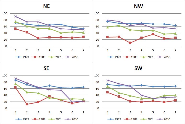
Spatial patterns of urbanisation: Spatial dynamic pattern of urban growth has been analyzed for 4 decades using eight landscape level metrics computed zone wise for each circle of 1 km radius. These metrics are discussed below:
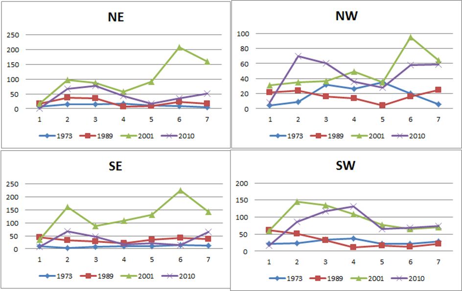
Number of Urban Patch (Np) , a landscape metric indicates the level of fragmentation and ranges from 0 (fragment) to 100 (clumpiness).
Fig. 8a illustrates the temporal dynamics of number of patches. Urban patches are less at the center in 1970’s as the growth was concentrated in central pockets. There is a gradual increase in the number of patches in 80’s and further in 2001, but these patches form a single patch during 2010, indicating that the urban area get clumped as a single patch at the center, but in the buffer regions there has been a tremendous increase in 2001. Clumped patches at center are more prominent in NE and SE directions and patches are agglomerating to a single urban patch.
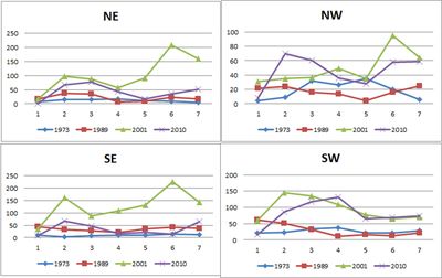
Fig. 8a. Number of urban patches (zonewise, circlewise)
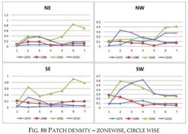
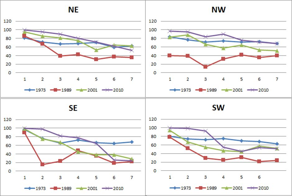
The patch density (Fig. 8b) calculated on a raster map, using a 4 neighbor algorithm, increases with a greater number of patches within a reference area. Patch density was higher in 1989 and 2001 as the number of patches was higher all the directions. Density declined at the central gradients in 2010. In the outskirts the patch density has increased in early 2000’s, which is indicative of sprawl in the region and PD is low at center indicating the clumped growth during late 2000’s, which is in accordance with number of patches.
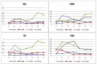
Fig. 8b. Patch density – zonewise, circle wise
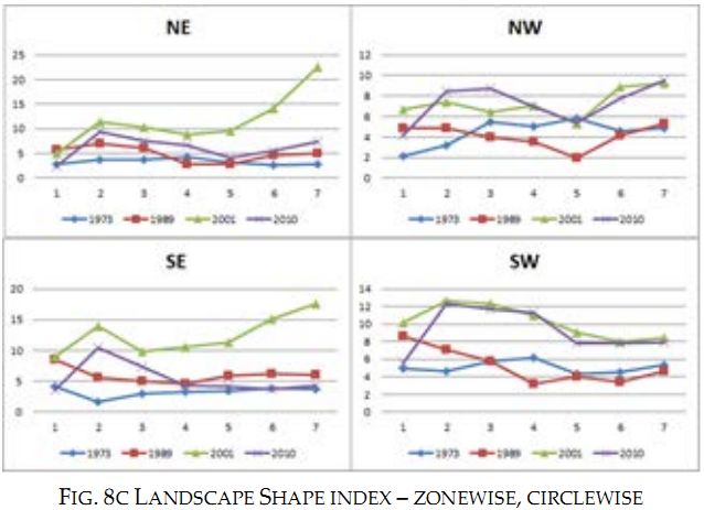
Landscape Shape Index (LSI): LSI is equal to 1 when the landscape consists of a single square or maximally compact (i.e., almost square) patch of the corresponding type and LSI increases without limit as the patch type becomes more disaggregated. Results (Fig. 8c) indicated that there were low LSI values in 1973 due to minimal and concentrated urban areas in the center. Since 1990’s the city has experienced dispersed growth in all direction and circles, towards 2010 it showed a aggregating trend at the center as the value was close to 1, whereas it was very high in the outskirts indicating the peri-urban development.
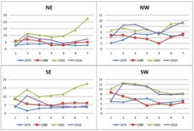
Fig. 8c. Landscape Shape index – zonewise, circlewise
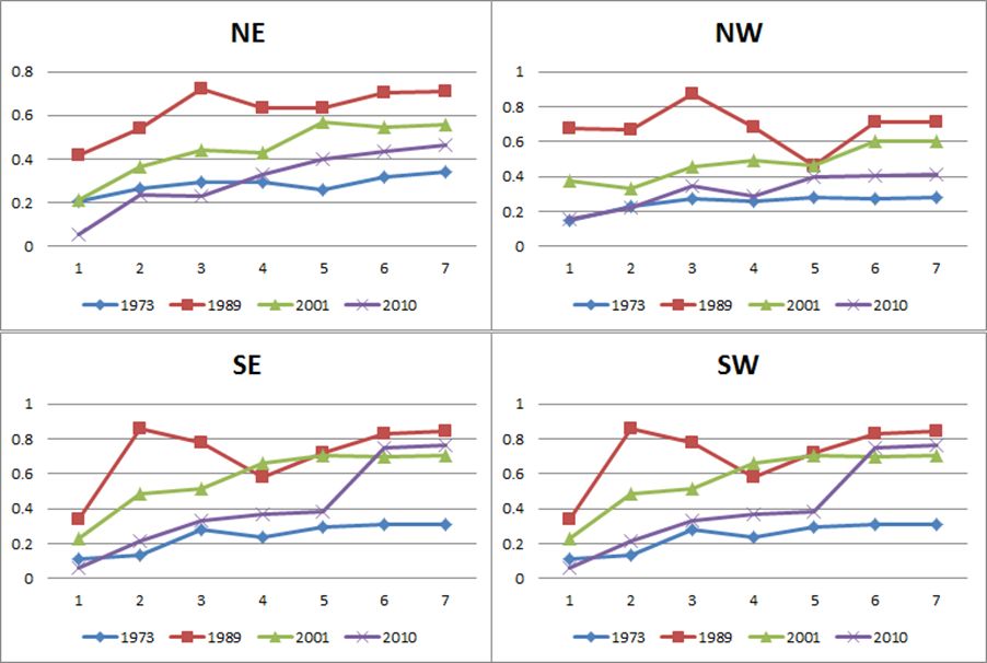
Normalized Landscape Shape Index (NLSI): NLSI is 0 when the landscape consists of Single Square or maximally compact almost square, and increases as patch types becomes increasingly disaggregated while it is 1 when the patch type is maximally disaggregated. Results (Fig. 8d) indicate that the landscape in 2010 had a highly fragmented urban class in the buffer region and is aggregated class in the center, in accordance with the other landscape metrics.
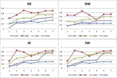
Fig. 8d. Normalised Landscape Shape index – zonewise, circlewise
Clumpiness index equals 0 when patches are distributed randomly, and approaches 1 when the patch type is maximally aggregated. Aggregation index equals 0 when patches are maximally disaggregated and equals 100 when the patches are maximally aggregated into a single compact patch.
Clumpiness and aggregation indices exhibit similar temporal trends and highlights that the center of the city is more compact in 2010 with more clumpiness and aggregation in NW and NE directions. In 1973 the results indicated that there were a small number of urban patches existing in all direction and in every circle. Post 2000 and in 2010, a large number of urban patches close to each other almost form a single patch especially at the center and in NW and NE direction in different gradients (Fig. 8e, Fig. 8f).
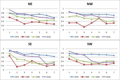
Fig. 8e. Clumpiness – zonewise, circle wise
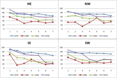
Figure 8f: Aggregation-zone and circle wise
Lower values of these metrics in the outer circles indicate that there is a tendency of sprawl in the outskirts.
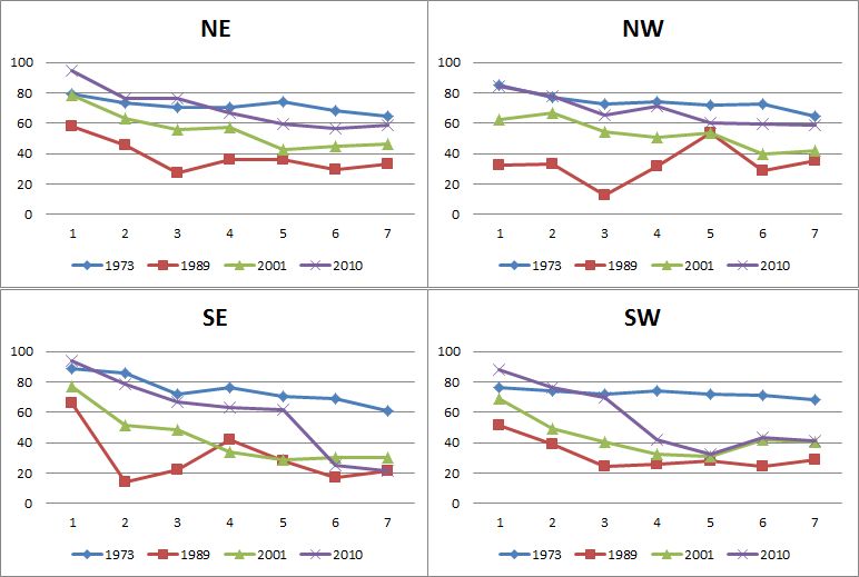
Percentage of Like Adjacencies (Pladj), the percentage of cell adjacencies involving the corresponding patch type are like adjacent. This metrics also indicates (Fig. 8g) that the city center gets more and more clumped and the adjacent patches of urban much closer have formed a single patch in 2010 and outskirts relatively sharing different internal adjacencies with patches not immediately adjacent but have a trend to become adjacent to each other, which is also indicative of sprawl.
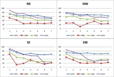
Figure 8g: Zone and circle wise: Pladj
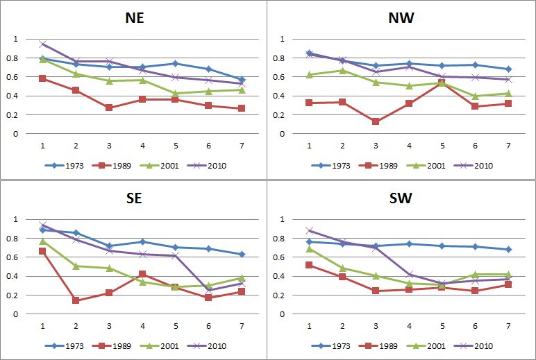
Patch cohesion index measures the physical connectedness of the corresponding patch type. Fig. 8h indicates physical connectedness of the urban patch with higher cohesion value (in 2010). Lower values in 1973 illustrated that the patches were rare in the landscape.
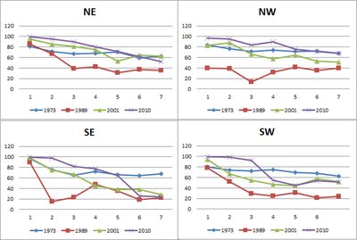
Figure 8h: Cohesion Index
|