|
Urbanisation and sprawl in the Tier II City: Metrics, Dynamics and Modelling using Spatio-Temporal data
|
 |
1Energy & Wetlands Research Group, Centre for Ecological Sciences [CES], 2Centre for Sustainable Technologies (astra), 3Centre for infrastructure, Sustainable Transportation and Urban Planning [CiSTUP],
Indian Institute of Science, Bangalore – 560012, India.
*Corresponding author: cestvr@ces.iisc.ac.in
|
METHOD
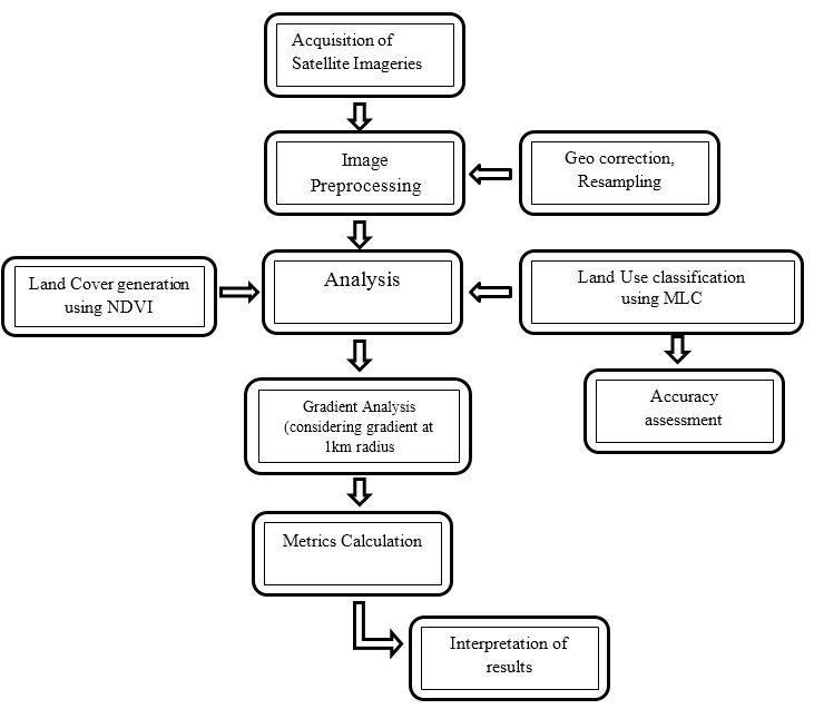
A stepwise normative gradient approach was adopted to understand the dynamics of the city, including (i) first step to derive land use and land cover (ii) a zonal-gradient approach of 4 zones and 1km radius gradients to understand the pattern of growth during the past 4 decades. (iii) understanding the change in the land use dynamics using Landscape metrics analysis. Various stages in the data analysis are as shown in Fig. 2.
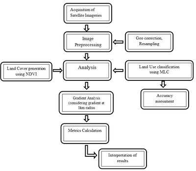
Figure 2: Procedure to understand the changes in spatial pattern and its dynamics
-
Preprocessing: The remote sensing data of landsat were downloaded from GLCF (Global Land Cover Facility) and IRS LISS III data were obtained from NRSC, Hyderabad. The data obtained were geo-referenced, rectified and cropped pertaining to the study area. The satellite data were enhanced using histogram equalization for the better interpretation and to achieve better classification accuracy. Furthermore, the images including topographical sheet and ward map were rectified to a common Universal Traverse Mercator (UTM) projection/co-ordinate system. All data sets were resampled to 30m spatial resolution using the nearest neighborhood re-sampling technique.
-
Vegetation Cover Analysis: Vegetation cover analysis was performed using the index Normalized Difference Vegetation index (NDVI) that was computed for all the years to understand the change in the temporal dynamics of the vegetation cover in the study region. NDVI value ranges from -1 to +1, where -0.1 and below indicates soil or barren areas of rock, sand, or urban built-up. NDVI of zero indicates the water cover. Moderate values represent low density vegetation (0.1 to 0.3) and higher values indicate thick canopy vegetation (0.6 to 0.8).
-
Land use analysis: Further to investigate the different changes in the landscape land use analysis was performed. Categories listed in Table II, were classified with the training data (field data) using Gaussian maximum likelihood supervised classifier. This analysis includes generation of False Color Composite (bands – green, red and NIR), which basically helps in visualization of the different heterogeneous patches. The further use of the training data Polygons were digitized corresponding to the heterogeneous patches covering about 40% of the study region and uniformly distributed over the study region. These training polygons were loaded in pre-calibrated GPS (Global position System). Attribute data (land use types) were collected from the field with the help of GPS corresponding to these polygons. In addition to this, polygons were digitized based on Google earth (www.googleearth.com) and Bhuvan (bhuvan.nrsc.gov.in). These polygons were overlaid on FCC to supplement the training data to classify landsat data.
Table II: Land use categories
| Land use Class |
Land uses included in the class |
| Urban |
This category includes residential area, industrial area, and all paved surfaces and mixed pixels having built up area. |
| Water bodies |
Tanks, Lakes, Reservoirs. |
| Vegetation |
Forest. |
| Cultivation |
Croplands, Nurseries, Rocky area. |
Gaussian maximum likelihood classifier (GMLC) is applied to classify the data using the training data, in which various classification decisions are involved by means of probability and cost functions [30] and is proved superior compared to other techniques. Mean and covariance matrix are computed using estimate of maximum likelihood estimator. Estimations of temporal land uses were done through open source GIS (Geographic Information System) - GRASS (Geographic Resource Analysis Support System, http://ces.iisc.ac.in/grass). 70% of field data were used to classify the data and the balance 30% were used in validation and accuracy assessment. Thematic layers were generated for the study region corresponding to four land use categories.
Evaluation on the performance of classifiers has been done through accuracy assessment techniques to test the statistical significance of a difference, comparison of kappa coefficients and proportion of correctly allocated classes through computation of confusion matrix. These are most commonly used to demonstrate the effectiveness of the classifiers [27][28].
-
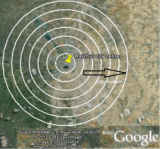
Further each zone was divided into concentric circle of increment radius of 1 km (Fig. 2.) from the center of the city to visualize the changes at neighborhood levels. This also helped in identifying the causal factors and the degree of urbanization (in response to the economic, social and political forces) at local levels and visualizing the forms of urban sprawl.
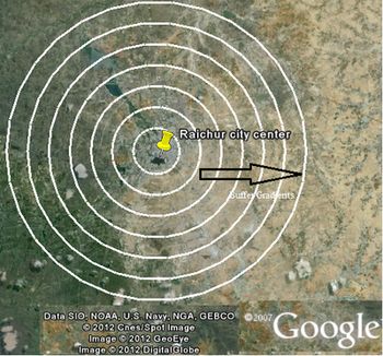
Fig. 2. Google earth representation of the study region along with the gradients
-
Urban sprawl analysis: Shannon’s entropy (Hn) is computed (equation 1) direction-wise to understand the extent of growth: compact or divergent. This provides an insight into the development (clumped or disaggregated) with respect to the geographical parameters across ‘n’ concentric regions in the respective zones.
 …… (1) …… (1)
Where Pi is the proportion of the built-up in the ith concentric circle and n is the number of circles/local regions in particular direction. Shannon’s Entropy values ranges from zero (maximally concentrated) to log n (dispersed growth).
-
Spatial pattern analysis: Landscape metrics provide quantitative description on the composition and configuration of the urban landscape. These spatial metrics have been computed for each circle, zone wise with the help of FRAGSTATS [18] using classified land use data at the landscape level. Urban dynamics is characterized with 7 prominent spatial metrics chosen based on complexity, and density criteria. The metrics including the patch area, shape, epoch/contagion/dispersion are listed in Table III.
Table III: Temporal Land cover details
| Year |
Vegetation (%) |
Non vegetation (%) |
| 1975 |
96.32 |
3.68 |
| 1989 |
92.18 |
7.82 |
| 2001 |
89.36 |
10.64 |
| 2010 |
82.48 |
17.52 |
|
|
Citation : Ramachandra. T.V. and Bharath H. Aithal, 2013, Urbanisation and sprawl in the Tier II City: Metrics, Dynamics and Modelling using Spatio-Temporal data., International Journal of Remote Sensing Applications (IJRSA),
Vol. 3, Issue 2, June 2013, pp. 66-75.
|