|
Results and Discussion
Land use analysis: Land use analysis was done using Maximum Likelihood classifier (MLC) considering training data collected from field. Land use analysis show an increase in urban area from 49915.42 (2008) to 59103 hectares (2012) which constitute about 30%. Fig. 3 illustrates the increase in urban area and the same is listed in table 4. Land use changes are due to various agents that have played role in urban growth. These agents include large IT sectors (in south east), Bangalore international airport (north east), several industrial areas (west and south west), etc. Gradual increase urban aggregations at periphery is noticed due to large availability of land at affordable price.
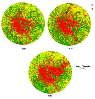
Fig. 3. Land use transitions during 2008 to 2012
Table 4: Land use during 2008, 2010 and 2012
Class
Year |
Built-up Area |
Water |
| Ha |
% |
Ha |
% |
| 2008 |
49915.42 |
24.85 |
1068.94 |
0.53 |
| 2010 |
57208.40 |
28.48 |
1571.41 |
0.78 |
| 2012 |
59103.90 |
29.33 |
1169.82 |
0.58 |
Class
Year |
Vegetation |
Others |
| Ha |
% |
Ha |
% |
| 2008 |
77036.96 |
38.35 |
72851.95 |
36.27 |
| 2010 |
73460.57 |
36.57 |
68,656.40 |
34.17 |
| 2012 |
67883.85 |
33.68 |
73385.73 |
36.41 |
Accuracy assessment: Accuracy assessment of land use analysis was performed by generating the reference image through the 30% of training data. Overall accuracy and Kappa was calculated using the module r.kappa in GRASS. The results of accuracy assessment are as shown in table 5.
Visualising the urban growth by 2020: Urban data (2008, 2010) were used as input to the land change modeller. MLP, was used to obtain transition considering various agents. The markov module provided the transition probability matric and finally growth for 2012 is predicted through CA_Markov (Fig. 4). The module was trained until the optimum accuracy was reached with good kappa value (Table 6). This module was optimized and calibrated to the evolving agents with urban change patterns.Considering the agents and the training data, prediction for the year 2020 was performed and given in Fig. 5 and table 7.
Table 5: Accuracy assessment
| Year |
Overall accuracy % |
Kappa |
| 2008 |
86.35 |
0.78 |
| 2010 |
91.62 |
0.86 |
| 2012 |
90.43 |
0.85 |
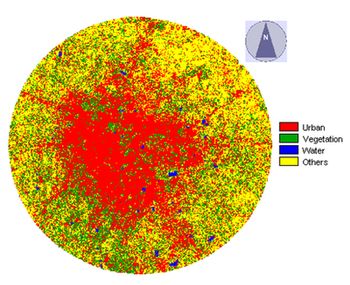
Fig. 4. Growth in 2012 (predicted) Bangalore
Table 6: Comparison of predicted land use with actual land use of 2012 -accuracy and kappa statistics
Class
Year |
Built-up Area |
Water |
Vegetation |
Others |
| % |
% |
% |
% |
| 2012 classified |
29.33 |
0.58 |
33.68 |
36.41 |
| 2012 predicted |
31.13 |
0.6 |
29.42 |
38.85 |
Overall accuracy:93.64, Kappa:0.91,Kloc: 0.9265,
Kno:0.8938, Kstandard:0.8874 |
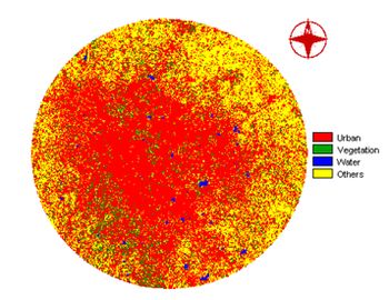
Fig. 5: Predicted growth of Bangalore by 2020 using LCM
Table 7: Land use statistics of Bangalore for 2020
Class
Year |
Built-up Area |
Water |
Vegetation |
Others |
| % |
% |
% |
% |
| 2020 Predicted |
61.27 |
0.55 |
7.00 |
31.18 |
The predicted land use reveals of similar patterns of urbanisation of last decade. The main concentration will be mainly in the vicinity of arterial roads and proposed outer ring roads. Predicted land use also indicate of densification of urban utilities near the Bangalore international airport limited (BIAL) and surroundings. Further an exuberant increase in the urban paved surface growth due to IT Hubs in south east and north east. The results also indicated the growth of suburban towns such as Yelahanka, Hesaragatta, Hoskote and Attibele with urban intensification at the core area. The predicted urban area is about 123,061.59 hectares (62%), a considerable increase of 208 times by 2020 (compared to 2012). This highlights the need for appropriateinfrastructure to cope up with the visualized growth to minimize drudgery to the common public.
Landscape metrics and urban analysis: Landscape metrics were calculated using Fragstat software to understand the extent of urban growth, its characteristics such as shape and contagion, etc.
Number of urban patches (NP): NP signifies the urban class growth in the landscape. It explains the kind of growth (patched/fragmented or unpatched/clumped) in the considered region. The results of this metric explains that there was increase in number of patches from 2008 to 2012, this signifies that there was a patched/fragmented growth. Post 2012 (Fig. 6) the NP decreases which indicates that there will be coalescence of grown urban patches to a single patch. Thus by 2020 urban densification is evident with the loss of other land uses.
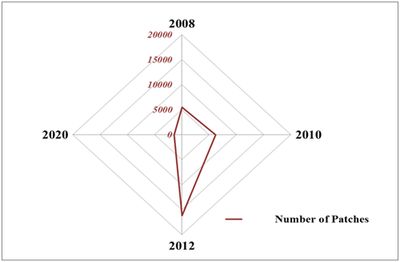
Fig. 6. Number of urban patches
Normalized landscape shape index (NLSI): This measures the shape of the class in the landscape and NLSI = 0 when the landscape consists of a single square or maximally compact and reaches 1 if the class becomes increasingly disaggregated or fragmented or shows convoluted shapes. This highlights of clumped growth by 2020 in conformity to the reduction of NP. Fig. 7 highlights the consolidation of urban patched to a clump.
Clumpiness index: Clumpiness index is a measure of adjacency indicating the extent of clumped or fragmentations in the urban growth. This values ranges from -1 (complete disaggregation) to 1 (maximal aggregation) and values near to 0 indicates of random distribution of patches. This index also indicates of highly concentrated aggregated clumped growth by 2020 (Fig. 7).
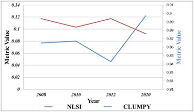
Fig. 7. Normalized landscape shape index and Clumpiness index
Edge density: Edge density is also a fragmentation index, which counts the edges formed by forming new classes in the landscape, the edge density increases between 2008 to 2010 indicative of fragmented growth and during 2010 to 2020 declines, indicative of clumped growth (Fig. 8).
Percentage of land adjacencies (PLADJ): This index shows how adjacent are the same features, based on neighborhood adjacencies. Values close to 100 shows the adjacent growth (with disappearance of other land uses), values close to 0 indicates of the presence of heterogeneous landscape with all land use categories. Values close to 100 in 2020 is indicative of adjacent clumped growth in the region (Fig. 8).
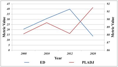
Fig. 8. Edge density and Percentage of land adjacencies
These spatial metrics highlight of aggregated growth by 2020 and the formation of concrete jungle with the disappearance of all other land uses. This haphazard growth would fuel unsustainability with the decline of vegetation, etc.
|
