|
Method
Modelling of urbanization and sprawl as outlined in Fig. 2, involved
- Remote Sensing data acquisition, geometric correction, field data collection,
- Classification of remote sensing data and accuracy assessment using GRASS,
- Identification of agents and development of attribute information using MapInfo,
- Designing three scenarios of urban growth and calibrating the model to find out the best weights based on the influence on the neighborhood pixels,
- accuracy assessment and validation of the model,
- Prediction of future growth based on validated data
- Computation of spatial metrics and analysis.
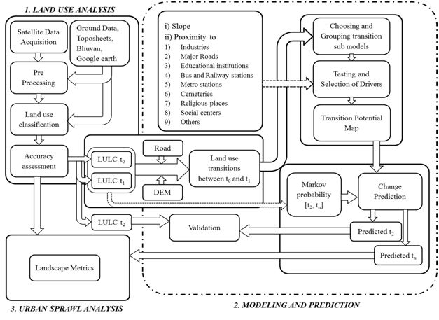
Fig. 2. Spatio-temporal analysis procedure
Image pre-processing: The remote sensing data of Landsat TM with spatial resolution of 30 m were acquired from USGS. These data were geometrical corrected using polynomial transformations and pre-processed for noise removal.
Land use analysis: Analysis was carried out using supervised pattern classifier - Gaussian maximum likelihood algorithm. This method has already been proved as a superior method as it uses various classification decisions using probability and cost functions [17]. Mean and covariance matrix are computed using estimate of maximum likelihood estimator. Four major types of land use classes were considered: built-up area, vegetation, open area, and water body as described in table 2. The method involves a) generation of false colour composite (FCC) of remote sensing data (bands – green, red and NIR). This helped in locating heterogeneous patches in the landscape b) selection of training polygons (these correspond to heterogeneous patches in FCC) covering 15% of the study area and uniformly distributed over the entire study area, c) loading these training polygons co-ordinates into pre-calibrated GPS, d) collection of the corresponding attribute data (land use types) for these polygons from the field. GPS helped in locating respective training polygons in the field, e) supplementing this information with Google Earth f) 60% of the training data has been used for classification of the data, while the balance is used for validation or accuracy assessment.
Table 2: Land use categories
| Land use Class |
Land use included in class |
| Urban |
Residential Area, Industrial Area, Paved surfaces, mixed pixels with built-up area |
| Water |
Tanks, Lakes, Reservoirs, Drainages |
| Vegetation |
Forest, Plantations |
| Others |
Rocks, quarry pits, open ground at building sites, unpaved roads, Croplands, Nurseries, bare land |
Training data was collected in order to classify and also to validate the results of the classification. Land use analysis was carried out with supervised classification scheme using training data. The supervised classification approach is adopted as it preserves the basic land cover characteristics through statistical classification techniques using a number of well-distributed training pixels. Maximum likelihood algorithm is a common, appropriate and efficient method in supervised classification techniques by using availability of multi-temporal “ground truth” information to obtain a suitable training set for classifier learning. Supervised training areas are located in regions of homogeneous cover type. All spectral classes in the scene are represented in the various subareas and then clustered independently to determine their identity. GRASS GIS (Geographical Analysis Support System) an open sourcesoftware has been used for the analysis, which has the robust support for processing both vector and raster files accessible at [18]
Accuracy assessment: Accuracy assessments decide the quality of the information derived from remotely sensed data. The accuracy assessment is the process of measuring the spectral classification inaccuracies by a set of reference pixels. These test samples are then used to create error matrix (also referred as confusion matrix), kappa (κ) statistics and producer's and user's accuracies to assess the classification accuracies. Kappais an accuracy statistic that permits us to compare two or more matrices and weighs cells in error matrix according to the magnitude of misclassification [1,2].
Modelling Land use scenario: Land use Change Modeller (LCM), an ecological modeller was used for modelling the land use scenario based on the data of 2008, 2010 and 2012. LCM module provides quantitative assessment of category-wise land use changes in terms of gains and losses with respect to each land use class. This can also be observed and analysed by net change module in LCM. The Change analysis was performed between the images of 2008 and 2010, 2010 and 2012, to understand the transitions of land use classes during the years. Threshold of greater than 0.1 ha were considered for transitions. CROSSTAB was used between two images to generate a cross tabulation table in order to see the consistency of images and distribution of image cells between the land use categories. Multi-Layer perceptron neural network was used to calibrate the module and relate the effects of agents considered and obtain transition potential sub models. Further markov module was used to generate transition probabilities, which were used as input in cellular automata for prediction of future transitions. This has been analysed LCM or using the CA_Markov.
Validation: Land use of 2012 was predicted using land use transition during 2008 to 2010 considering 2008 as base year. The predicted 2012 land use was compared with classified land use of 2012 (based on remote sensing data of 2012). This was repeated with 2010 data as base year considering the transition during 2010 to 2012. Validation was performed using validate, calculating Kappa, Kloc, Kno, Kstandardfor simulated images and classified image of 2012. Similarly,prediction for 2020 was done considering 2010 and 2012 as base images.
Spatial pattern analysis: Spatial metrics provide quantitative description of the composition and configuration of urban landscape. These metrics were computed for classified land use data at the landscape level using FRAGSTATS. Urban dynamics is characterized by select spatial metrics [1,3,11,13] listed in Table 3, chosen based on shape, edge, complexity, and density criteria. The metrics include the patch area, shape, epoch/contagion/ dispersion.
Table 3: Landscape metrics analysed
| |
Indicators |
Formula |
| 1 |
Number of Urban Patches (NPU) |

NP equals the number of patches in the landscape. |
| 2 |
Normalized Landscape Shape Index (NLSI) |

Where siand pi are the area and perimeter of patch i, and N is the total number of patches. |
| 3 |
Total Edge (TE) |
 ik ik
where, eik = total length (m) of edge in landscape involving patch type (class) i; includes landscape boundary and background segments involving patch type i. |
| 4 |
Clumpiness index(Clumpy) |

Range: Clumpiness ranges from -1 to 1 |
| 5 |
Percentage of Land adjacency (Pladj) |
gii = number of like adjacencies (joins) between pixels of patch type gik = number of adjacencies between pixels of patch types i and k
Range: 0<=PLADJ<=100 |
|
