 |
Urbanization in India: Patterns,Visualization of Cities, and Greenhouse Gas Inventory for Developing Urban Observatory
|
 |
aRCGSIDM, Indian Institute of Technology Kharagpur, West Bengal, India bEnergy and Wetland Research Group, Centre for Ecological Science, Indian Institute of Science, Karnataka, India
*Corresponding author: bhaithal@iitkgp.ac.in
Result and Outcomes
4.1. Land Use Analysis
Land use for different time periods was assessed using GML classifier. Dramatic changes in the landscape of various parts of India for over three decades are shown in Figure 7.3. Mumbai has shown a significant increase in built-up areas from 3.32% in 1973 to 14.26% in 2009. An extensive decrease of 74% can be seen in vegetation category from 1973 to 2009. In terms of urbanization and urban sprawl, Delhi is no different from Mumbai, since it also shows an increase in impervious urban areas from 3.6% to 25.06% over a period of 33 years. This tremendous change in landscape makes surrounding places more vulnerable to various hazards and issues such as ecological imbalance (Riley et al. 2005; Xian et al. 2007), change in rainfall pattern leading to urban floods (Bronstert et al. 2002; McCuen and Beighley 2003), formation of urban heat island, traffic density congestion and therefore increases in air pollution, stress on surface as well as subsurface water resource, and so on. Further, density gradient analysis showed agents that fueled rapid urban growth in and around the Indira Gandhi International Airport (IGI) and the Indian Air Force base (Hindon). Classification results for Kolkata indicate a steep increase in urban category, which occurred at the cost of wetland and agriculture land degradation in various places (Ramachandra et al. 2014c).
Results for the Chennai region revealed a surge in built-up areas of 72% (1991–2000) and 646% (2000–2013). It is necessary to note that the growth that occurred especially in 2000 and 2010 is attributed to industrial and information technology policy measures. Industries play a key role in the urban growth process by attracting a huge number of populations from core city areas to urban fringe or transition zones; these zones later become part of a greater city region. Land use results for the Bangalore region shows a twofold increase in urban area from 24.86% to 48.39% within a span of 4 years (2008–2012). During this period, Bangalore lost a huge amount of trees especially due to pressure from construction of buildings, expansion of roadways, introduction of the metro-rail system, and so on. The vegetation cover decreased from 38.34% to 26.40%, showing unplanned urban growth.
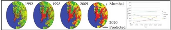
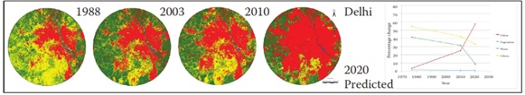
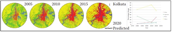
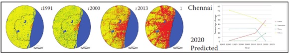
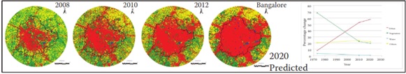
Figure 7.3 Temporal landscape dynamics of study regions.
4.2. Validation
Accuracy assessment for land use classification was performed based on kappa statistics and overall accuracy as shown in Table 7.4. The results of overall accuracy indicate that classified maps along with ground truth have a lot of resemblance and are therefore accurate.
| City |
Mumbai |
Delhi |
Chennai |
Kolkata |
Bangalore |
| Year |
1992 |
1998 |
2009 |
1988 |
2003 |
2010 |
1991 |
2010 |
2013 |
2005 |
2010 |
2015 |
2008 |
2010 |
2012 |
| Overall accuracy (%) |
73 |
99 |
97 |
99 |
88 |
91 |
92 |
91 |
97 |
88 |
93 |
91 |
94 |
98 |
97 |
| Kappa |
0.81 |
0.82 |
0.81 |
0.99 |
0.84 |
0.96 |
0.92 |
0.9 |
0.9 |
0.9 |
0.99 |
0.96 |
0.98 |
0.96 |
0.95 |
Table 7. 4 Overall Accuracy and Kappa Statistics
4.3. Modeling and Prediction
Land use transitions were calculated to determine land use change for the year 2020 for Mumbai, Delhi, Kolkata, Chennai, and Bangalore. Markov chain was used to derive probability of change between two time periods. Knowing the land use of T 0 and T1, the land use of time period T 2 was predicted. Prediction was made considering important urbanizing agents such as industries, educational institutes, road network, rail network, hospitals, and other service facilities. Constraints such as water bodies, wetland areas, protected areas, and so on were assumed to remain constant over all periods of time. Predicted results for time T2 were compared with classified maps for time period T2 to validate the data sets. Predicted maps were observed to be in good agreement, obtaining high accuracy and kappa values. Therefore, the process was repeated to predict land use for the period Tn. Cities like Delhi and Kolkata have shown a twofold increase in paved areas from time period T2to Tn. Density and gradient analysis for the predicted areas confirmed that core urban areas are clumped as one large built-up patch, thereby not giving any other category the chance to develop.
4.4. Transition Probability
Based on land use during T 1and T2, Markov transition potentials were computed, and the probability matrices of each land use type are given in Table 7.5. Diagonal elements indicative of land use classes being the same and other elements indicate the probability of land use to transition into land use classes. The results for most of the cities and built-up areas remain almost constant; non-urban land use classes have a higher probability of transitioning into an urban land use class. Bangalore showed substantial loss of water bodies and vegetation (as also reported by Ramachandra et al. 2017; Ramachandra and Bharath 2016). Kolkata and Chennai also follow the same trend.
| Markov Transition Probabilities for Mumbai for the Period 1998–2009 |
| |
|
Built-Up Areas |
Water Bodies |
Vegetation |
Others |
| 1998–2009 |
Built-up areas |
0.990 |
0.000 |
0.000 |
0.010 |
| Water bodies |
0.332 |
0.634 |
0.030 |
0.004 |
| Vegetation |
0.486 |
0.003 |
0.475 |
0.036 |
| Others |
0.623 |
0.001 |
0.002 |
0.374 |
| Markov Transition Probabilities for Delhi for the Period 2003–2010 |
| 2003–2010 |
Built-up areas |
0.970 |
0.000 |
0.002 |
0.028 |
| Water bodies |
0.38 |
0.604 |
0.008 |
0.008 |
| Vegetation |
0.528 |
0.001 |
0.431 |
0.04 |
| Others |
0.613 |
0.001 |
0.018 |
0.368 |
| Markov Transition Probabilities for Kolkata for the Period 2010–2015 |
| 2010–2015 |
Built-up areas |
0.992 |
0.000 |
0.000 |
0.008 |
| Water bodies |
0.18 |
0.754 |
0.005 |
0.061 |
| Vegetation |
0.612 |
0.001 |
0.386 |
0.001 |
| Others |
0.693 |
0.000 |
0.006 |
0.301 |
| Markov Transition Probabilities for Bangalore for the Period 2010–2015 |
| 2008–2012 |
Built-up areas |
0.998 |
0.000 |
0.000 |
0.002 |
| Water bodies |
0.604 |
0.386 |
0.004 |
0.006 |
| Vegetation |
0.793 |
0.001 |
0.177 |
0.029 |
| Others |
0.486 |
0.002 |
0.006 |
0.506 |
| Markov Transition Probabilities for Chennai for the Period 2010–2015 |
| 2008–2012 |
Built-up areas |
0.948 |
0.000 |
0.030 |
0.022 |
| Water bodies |
0.326 |
0.645 |
0.008 |
0.021 |
| Vegetation |
0.516 |
0.000 |
0.467 |
0.017 |
| Others |
0.294 |
0.004 |
0.013 |
0.689 |
Table 7. 5 Markov Transitional Probability for Study Regions
4.5.GHG Footprint
Results from the energy sector revealed that Delhi has the highest commercial CO2e emission. The Delhi region consumed 5339.63 MU of electricity during 2009–2010, releasing 5428.55 Gg of CO2. The Kolkata region, which released approximately 1746.34 Gg of CO2, contributed the least among the five cities. Delhi also showed maximum CO2e for the domestic sector, with 11,690.43 Gg, followed by Chennai (8617.29 Gg), Greater Mumbai (8474.32 Gg), Kolkata (6337.11 Gg), and Bangalore (4273.81 Gg). Transportation sector emissions were recorded for vehicles using fuel CNG and nonCNG separately. The lowest value under this sector was for the Kolkata region, with 1886.60 Gg of emission from the non-CNG category only, whereas the peak values were observed for the Delhi region with 10,867.51 Gg under the non-CNG category and 1527.03 under CNG vehicles. The industry sector emission results revealed that ammonia production and fertilizer industries in Greater Mumbai and Chennai yielded 654.5 and 223.28 Gg of CO 2e, respectively. The Delhi region had a large amount of CO 2 e emission from the agriculture sector (17.05 Gg from paddy cultivation, 248.26 Gg from soils, and 2.68 Gg from crop residue burning), followed by Bangalore (5.10 Gg from paddy cultivation and 113.86 Gg from soils). The livestock management and waste sector also had similar results, where Delhi was at the peak in terms of CO 2e emission followed by other regions. The combination of all these sectors clearly indicates that the range varies from 38,633.20 Gg/year (Delhi region) to 14,812.10 Gg/year (Kolkata region). Furthermore, sector-wise analysis shows that, of all the considered sectors, the transportation sector (Delhi, 32.08%; Bangalore, 43.48%) and the domestic sector (Mumbai, 37.20%; Chennai, 39.01%; Kolkata, 42.78%) have the highest emissions. The huge emissions from the transportation sector can be attributed to unplanned urbanization as well as to a lack of public transportation system, as a result of which people tend to use private vehicles. The results sector-wise are presented in Figure 7.4.
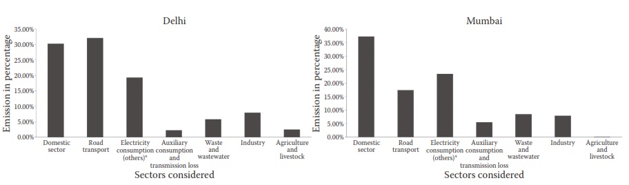
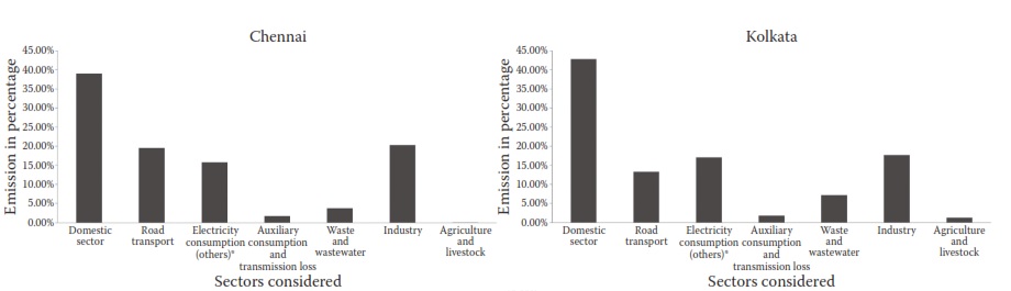
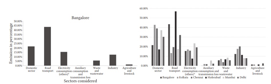
Figure 7.4 GHG Emissions Of Study Regions.
Citation : Bharath Haridas Aithal, Mysore Chandrashekar Chandan, Shivamurthy Vinay, T.V. Ramachandra, 2018, Urbanization in India: Patterns, Visualization of Cities, and Greenhouse Gas Inventory for Developing Urban Observatory. CRC Press Taylor & Francis Group 6000 Broken Sound Parkway NW, Suite 300 Boca Raton, FL 33487-2742 © 2018 by Taylor & Francis Group, LLC CRC Press is an imprint of Taylor & Francis Group, an Informa business.
| * Corresponding Author : |
|
Bharath Haridas Aithal
RCGSIDM, Indian Institute of Technology Kharagpur, West Bengal, India
Energy and Wetland Research Group, Centre for Ecological Science, Indian Institute of Science, Karnataka, India
E-mail : bhaithal@iitkgp.ac.in |
|
|
Bharath Haridas Aithal
aRCGSIDM, Indian Institute of Technology Kharagpur, West Bengal, India
bEnergy and Wetland Research Group, Centre for Ecological Science, Indian Institute of Science, Karnataka, India
* Corresponding Author
E-mail : bhaithal@iitkgp.ac.in
Mysore Chandrashekar Chandan
aRCGSIDM, Indian Institute of Technology Kharagpur, West Bengal, India
Citation:Bharath Haridas Aithal, Mysore Chandrashekar Chandan, Shivamurthy Vinay, T.V. Ramachandra, 2018, Urbanization in India: Patterns, Visualization of Cities, and Greenhouse Gas Inventory for Developing Urban Observatory. CRC Press Taylor & Francis Group 6000 Broken Sound Parkway NW, Suite 300 Boca Raton, FL 33487-2742 © 2018 by Taylor & Francis Group, LLC CRC Press is an imprint of Taylor & Francis Group, an Informa business.
Shivamurthy Vinay
bEnergy and Wetland Research Group, Centre for Ecological Science, Indian Institute of Science, Karnataka, India
|