 |
Urbanization in India: Patterns,Visualization of Cities, and Greenhouse Gas Inventory for Developing Urban Observatory
|
 |
aRCGSIDM, Indian Institute of Technology Kharagpur, West Bengal, India bEnergy and Wetland Research Group, Centre for Ecological Science, Indian Institute of Science, Karnataka, India
*Corresponding author: bhaithal@iitkgp.ac.in
Method
Figure 7.2 depicts the method adopted to assess urban growth patterns, which included three significant stages: data creation, land use and land cover analysis, and integrated model generation and validation.
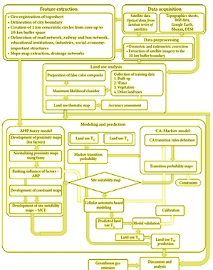
Figure 7.2 An Integrated Model Approach.
3.1 Data Creation
Data were obtained from a survey of India topographic sheets. The sheets with scales of 1:50,000 and 1:250,000 were scanned with high resolution. City administrative maps were obtained from the respective metropolitan development authority database. Ground truth data of various locations within the study region were taken using handheld GPS. Places that were inaccessible and remote were visualized using Google Earth and Bhuvan.
All these data sets corresponding to different study regions were geo-referenced and re-projected to common datum world geodetic system 1984 (WGS84) and respective UTM zones to ensure uniformity in mapping. Hence, region-specific administrative boundary maps were obtained. Further, a 10-km buffer was drawn from the centroid of the central business district to better understand the urbanization process beyond city administrative boundaries. Concentric circles of 1-km radius were also delineated from the centroid along with four major directional grids (i.e., NE, NW, SE, and SW) to analyze minute changes within these fragments.
3.2 Land Use Analysis
Satellite data for various time periods were geo-referenced (to WGS84 and respective UTM zones), geo-corrected, rectified, and cropped, pertaining to different study regions. To maintain similar resolution and for better comparison, satellite data were resampled to 30 m using nearest-neighborhood function. Land use analysis was performed to understand change in landscape pattern throughout the study regions temporally. It involved the following process:
(a) generation of a false color composite (FCC) image,
(b)digitizing training polygons using FCC as base layer to distinguish heterogeneous features,
(c) collection of training polygons via Google Earth (https://www.google.com/earth) (used as ancillary data for classification)
(d) classification using Gaussian Maximum Likelihood (GML) classifier
(e) validation and accuracy assessment. Land use analysis was performed using Geographical Analysis Support System open source software with four different categories as shown in Table 7.2.
A classification process is complete only when its accuracy is tested. Accuracy can be obtained by preparation of an error matrix or a confusion matrix (Congalton and Green 2008). User accuracy, producer accuracy, overall accuracy, and kappa statistics were calculated from the error matrix. Overall accuracy considers only diagonal elements of reference map and classified map, whereas kappa statistic takes into account off-diagonal elements as well (Lillesand et al. 2014).
| Category |
Features Involved |
| Built-up |
Houses, buildings, road features, paved surfaces, etc. |
| Vegetation |
Trees, gardens, and forest |
| Water body |
Seas, lakes, tanks, rivers, and estuaries |
| Others |
Fallow/barren land, open fields, quarry site, dry river/lake basin, etc. |
Table 7. 2 List of Different Categories Used for Land Use Analysis and Corresponding Features
3.3 Integrated Model Generation and Validation
Urbanizing agents and constraints were delineated in the form of points, lines, and polygons using Google Earth interface. Proximity maps were generated using minimum and maximum distance functions from each agent layer. Data values were normalized using fuzzy functions, and the entire range was between 0 and 255 (0 indicating no changes and 255 indicating maximum probability of change in land use types). The analytical hierarchical process was employed to estimate principal eigenvectors, and therefore, priority maps were created. Classified land use maps for initial stages, say, T0, T1, and T 2, were considered along with slope, and drainage layers analyzed using digital elevation model imageries were given as inputs to generate land use transitions from T 0 to T1 and from T1 to T2. Markov chain analysis was used to calculate the transition probability matrix based on two different time periods of classified images (Guan et al. 2008), where the probability of each land use type changing to the other remaining categories within the region considered is recorded after a specific number of iterations. Cellular automation with Markov chain was used to predict future land use for a specified year. Model validation was done by generating an error matrix for time period T2of both classified image versus simulated image.
3.4 Estimation of GHG Footprint
The method involved for calculating GHG can be divided into two significant steps. In the first step, a sector-wise approach was adopted to quantify GHG emissions. Various sectors and their description are given in Table 7.3. GHG footprint was calculated using equation factors and various attributes as per Ramachandra et al. 2015b.
The major GHGs that were taken into consideration were carbon dioxide CO2), methane (CH4), and nitrous oxide (N2O). The second step included the conversion of non-CO 2 gases into units of CO2 equivalent (CO2e), and the aggregation of CO2e was conducted as a region-specific analysis covering all the five study regions.
| Sl. no. |
Sector |
Description |
| 1 |
Energy sector: electricity consumption and fugitive emissions |
Combustion of fossil fuels in thermal power plants; gases occurring during extraction, production, processing, and transportation of fossil fuels. Gas emissions include CO2, SOx, NOx, SPM, and CH4. |
| 2 |
Domestic sector |
Major contribution from activities like cooking (using LPG, firewood, and kerosene), lighting, and heating and from household appliances. CO2, SOx, NOxand SPM. |
| 3 |
Transportation sector |
Emissions calculated by considering fuel consumed or distance traveled by various types of vehicles. Emissions from number ofvehicles using compressed natural gas (CNG) were also accounted for. CO 2, SOx, N2O and CH4 |
| 4 |
Industrial sector |
Major industries considered to emit CO2are iron and steel, ammonia manufacturing units, chemical products from fossil fuels, cement industry, petrochemical plants, fertilizer plants, power plants, glass industry, etc. |
| 5 |
Agriculture sector |
Includes paddy cultivation—the main phenomenon of CH4 emissions from rice fields to atmosphere, agricultural soils, and burning of crop residues. Gases quantified under this sector are CH4, N2O (direct and indirect emissions), NOx, and CO2 |
| 6 |
Livestock sector |
Chief activities listed under animal husbandry include enteric fermentation and manure management. CH 4 and N2O gases are calculated in this sector. |
| 7 |
Waste sector |
Methane is the major GHG emitted under the waste sector. The broad classes under waste can be listed as municipal solid waste disposal, domestic wastewater and industrial wastewater. Nitrous oxide (N2O) emissions can occur both directly (from wastewater treatment plants) or indirectly (from wastewater after disposal of effluent to water bodies). |
Table 7. 3 Sector-Wise GHG Emission and Description
Citation : Bharath Haridas Aithal, Mysore Chandrashekar Chandan, Shivamurthy Vinay, T.V. Ramachandra, 2018, Urbanization in India: Patterns, Visualization of Cities, and Greenhouse Gas Inventory for Developing Urban Observatory. CRC Press Taylor & Francis Group 6000 Broken Sound Parkway NW, Suite 300 Boca Raton, FL 33487-2742 © 2018 by Taylor & Francis Group, LLC CRC Press is an imprint of Taylor & Francis Group, an Informa business.
| * Corresponding Author : |
|
Bharath Haridas Aithal
RCGSIDM, Indian Institute of Technology Kharagpur, West Bengal, India
Energy and Wetland Research Group, Centre for Ecological Science, Indian Institute of Science, Karnataka, India
E-mail : bhaithal@iitkgp.ac.in |
|
|
Bharath Haridas Aithal
aRCGSIDM, Indian Institute of Technology Kharagpur, West Bengal, India
bEnergy and Wetland Research Group, Centre for Ecological Science, Indian Institute of Science, Karnataka, India
* Corresponding Author
E-mail : bhaithal@iitkgp.ac.in
Mysore Chandrashekar Chandan
aRCGSIDM, Indian Institute of Technology Kharagpur, West Bengal, India
Citation:Bharath Haridas Aithal, Mysore Chandrashekar Chandan, Shivamurthy Vinay, T.V. Ramachandra, 2018, Urbanization in India: Patterns, Visualization of Cities, and Greenhouse Gas Inventory for Developing Urban Observatory. CRC Press Taylor & Francis Group 6000 Broken Sound Parkway NW, Suite 300 Boca Raton, FL 33487-2742 © 2018 by Taylor & Francis Group, LLC CRC Press is an imprint of Taylor & Francis Group, an Informa business.
Shivamurthy Vinay
bEnergy and Wetland Research Group, Centre for Ecological Science, Indian Institute of Science, Karnataka, India
|