Results

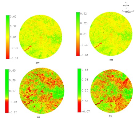
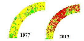
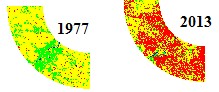
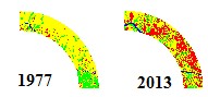
Land cover analysis: Land cover computed through NDVI, shows a decline of vegetation from 26.62% (1977) to 21.32% (2013) and year wise changes are tabulated in table 3 and depicted in Fig. 4.

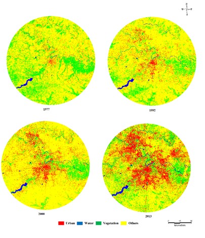
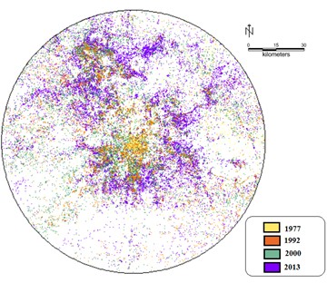
Land use analysis: Land use analysis was performed to classify into four categories through GMLC using training data collected from the field, Google earth and SOI toposheets. Fig. 5. The statistics calculated is as tabulated in table 4. The results show that the urban paved surface increased by around 689 times from 3% to 10%. The analysis showed the increase in vegetative cover which can be attributed to increase in agricultural area with crop. Water class remained fairly constant and other class which included open area, agricultural plots without crop decreased overtime from 73% to 60 %. Urban growth in past 4 decades in the study region can be seen in Fig. 6, this explains growth of urban land use in every decade. Assessment of land use dynamics helps in understanding the trends of urban expansions. This illustrates the maximum growth in South-East, North-East and North-West directions and occurs mainly in the gradients near the centre. Minimal growth or marginal growth compared to central gradients is seen in buffer zones and the periphery.

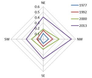
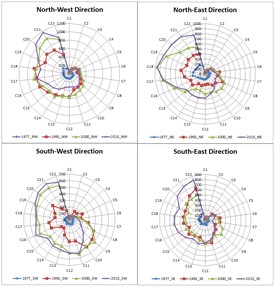
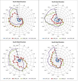
Accuracy assessment: Accuracy assessment of the classified images was done through the computation of overall accuracy and kappa statistics as shown in table 5. Overall accuracy ranges from 81% to 94%. Urban growth in each decade is as represented in Fig. 6. Shannon entropy: Shannon entropy was computed zone wise (by dividing the region into 4 parts based on cardinal directions and with one km incremental radius from the center). The Values close to log of the gradients in each direction explains that the region is completely fragmented and has experienced sprawl. The values close to zero indicated clumped central core growth. The results of the analysis are as shown in Fig. 6. The values show that there is influence sprawl in the region especially in NW and NE directions.

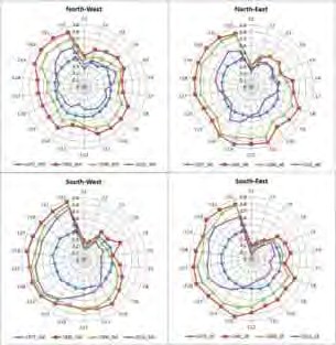
The values are as high as 0.52 in NW and 0.41 in NE are just midway of log (22) (22 gradients) = 1.3. Shannon Entropy highlights that the region is experiencing land transformation from centric growth to multidimensional fragmented growth. This growth might create more concentrated unconnected patch growths, leading to haphazard development without basic facilities, thereby impacting the local environment. This indicates that the region has to be monitored gradient wise to understand the specific pockets of growth that will help city managers to plan further developments (Fig. 7). Thus an analysis of landscape metrics gradient wise and zone wise was carried out. Spatial patterns of urbanisation: Spatial pattern of urbanization were assessed zone-wise for each gradient through select spatial metrics.

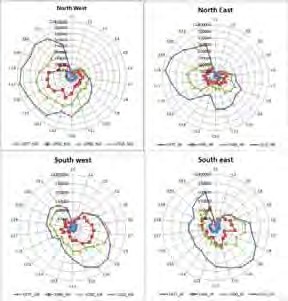
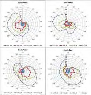
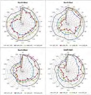
Number of Urban patches (NP) and Patch density (PD): These metric quantifies patches that helps to identify the level of fragmentation (Fig. 8a). Higher the number of patches, then the region is under fragmentation. Patch density analogous to NP reflects number of patches per unit area is given in Fig. 8(a) and Fig. 8(b). Highlights that Pune had clumped growth during 70’s and 90’s in all zones and confined to the core areas of the city. Post 2000 the city showed the signs of fragmentation especially in north-west and north-east directions with values reaching 500 patches in near periphery. Buffer zones also show similar trends with approximately 200 patches on an average, and 800 patches (2013) in all directions resulting in higher patch densities which indicates of sprawl in the region. Total edges and edge density: Edges and edge density basically are indicator of fragmentation in the landscape. Edge density represents denseness of the patches/edges in the landscape. Edges in 1977 across all zones and circles indicates that the core of the city are clumped. Further, post 1992 edges have increased highlighting fragmented out growth. In 2013, Gradients covering the inner core are clumped in the northeast and north-west directions, and the outskirts are with large number of edges (~300000 edges) in NW and NE directions. Density of 1.5 signify higher edges. Fig. 8c and 8(d) represents outputs of Total edge and Edge density.

Normalized shape index (NLSI): NLSI describes the shape of the particular class in the landscape. It is 0 when the landscape consists of a maximally compact patch and increases as the patch type becomes increasingly disaggregated and is 1 when the patch type is maximally disaggregated (Fig. 8(e)). The results of the analysis show that the gradients near the core with aggregations are forming a compact patch, whereas outer gradient in all direction with the spurt in urban activities show a value closer to 0.9 in almost all zones in the buffer zones indicating of sprawl as the shape of landscape is irregularly disaggregated and fragmented.

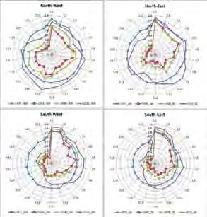
Cohesion index: Cohesion index implies the physical connectedness of the focal class and the value is 0 with the decline of the proportion of urban class in the landscape, which is indicative of fragmented outgrowth else increases monotonically, evident in Fig. 8f, indicating the emergence of urban sprawl in buffer zones and the decrease of the physical connectedness near the core similar to earlier metrics.

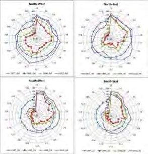
Clumpiness index (Clumpy) and Percentage of like adjacencies (Pladj): CLUMPY metric directly measure aggregation and disaggregation of the class in the landscape, equals -1 when the class is maximally disaggregated; and equals 0 when the class is distributed randomly, and approaches 1 when the patch type is maximally aggregated. PLADJ equals 0 when the focal class is maximally disaggregated and no like adjacencies and is equal to 100 when the focal class is a single patch is adjacent between same classes.

These metrics are dependent on adjacent characteristics of the focal class in the landscape. Fig. 8g and 8h shows that gradients reaching aggregation or single patch class from 1977 to 1992 in all zones. However, post 2000 the initiation of fragmentation value reaches 0 for Clumpy and Pladj signifying the fragmentation due to urban outgrowth. This phenomena can be mostly seen in the buffer zones and in regions under extreme pressures of sprawl.

Spatial metrics indicates of sprawl especially in the periphery and the buffer zones. These regions requires an immediate attention by the decision makers to provide appropriate infrastructure and basic amenities. Metrics computed in each temporal gradients equip the decision-makers with fundamental information about the growth, the role of agents (for example policy decisions to setup industrial layouts, etc.), rate of growth, spatial patterns of growth and information about site specific details such as patches or clumpiness or shapes in the landscape.

This knowledge helps in visualizing the extent and patterns of future growth, which helps in adopting strategies to control or mitigate potential impacts on the sustenance of natural resources due to large scale land cover changes.

Spatial pattern dynamics elucidation throws light on the role of earlier government policies (Fig. 9) in urban sprawl or urbanisation process in the region. This also helps in assessing the effectiveness of earlier urban policy measures to address sprawl and development of a city. Integrated management of natural resources involves understanding the rationale of development and making decisions of placing the regions specific development trajectory while maintaining the urban open spaces (parks, lakes, vegetation, etc.), natural water drains and resources.

Localities such as Pimpri, Chinchwad, Kahdakwasla, Dhayari phata, Katruj, Yerwada, Pashan, Lavale, Warje, Baner, Khadki, Tharwade, Pirangut etc., in and around Pune are experiencing large scale land cover changes due to the government push for industrialization in 1990’s are now facing the problem due to sprawl and associated problems such as lack of basic amenities, etc.

The spatial analyses establishes that gradient based metrics computation helps in understanding thespatial patterns of a dynamically evolving urban landscape (Keiner and Arley, 2007, Aguilera, 2008) like Pune given the momentum of growth and pressing need to characterize and plan in efficient manner. Fig. 9 illustrates the potential of gradient based spatial pattern analysis in understanding the land use dynamics due to policy interventions.

Pimpri Chinchwad was established in 1988 and developed to cater the requirement of industrial needs. This region is located in gradients 11, 12 and 13 in the north-west zone.

These gradients had higher vegetative cover in the pre-1990. But post 2000 it can be seen extensive conversion of vegetative area urban land use. Landscape metrics for this gradients show that the urban impervious surface were located as a continuous simple shape concentrated surface pre-2000 (Fig. 9a). Post 2000 these regions have experience significant land use change and conversion in to highly fragmented area. In 2013 these regions have changed into most fragmented gradients in North West zone.

Warje (Fig. 9b) is located close to periphery of the Pune municipal boundary. Gradient 6-9 represents this industrial region in the south west zone. The land use before 1990 was dominated by other land use class and post 2000 is dominated by the urban land use. Post 2000, the region formed a clumped simple patch, which indicates of prevalence of urban patch dominance.

Yerawada and Nagar road (Fig. 9c) is located in north east region of Pune and 7-8 gradient of North east zone and contribute about 10% to the industrial output of Pune. Landscape metrics of urban land use highlights that these gradients (post 2000) are in the verge of forming a single dominant urban class with simple shapes.

These spatial analyses confirm that policy and socio-economic factors fuel URBANIZATION. Urban planning require essential up-to-date knowledge of spatial patterns of land use changes to regulate and plan the city’s expansion as well as infrastructure development. Access to consistent and integrated spatial information about land use dynamics aids in the strategic understanding of the region specific growth for formulating effective cognitive decision on natural resources management by city planners with all stakeholders. Location specific information enhances the planning process through multitude of factors having decisive role in the land use sustainability.