Method
Spatial pattern of urbanisation is assessed using temporal remote sensing data of 1977 to 2013. The analysis is outlined in Fig. 3, which includes pre-processing, analysis of land cover and land use, and finally spatial patterns analysis through gradients and zones using spatial metrics. The study region includes Pune administrative area with 10 km buffer to account pockets at city outskirts experiencing sprawl.
Fig. 3: Procedure followed in analysis 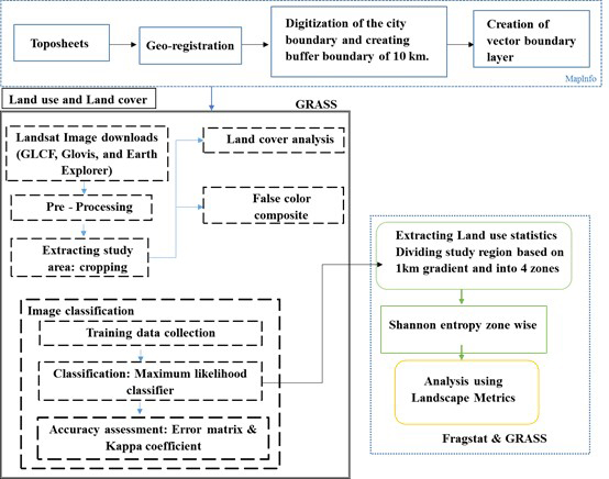 |
Pre-processing:
Remote sensing data (Landsat series) for Pune, acquired for different time periods, were
geo-corrected and cropped pertaining to the study area. Geo-registration of remote sensing data (Landsat data) has been done using ground control points collected from the field using pre calibrated GPS (Global Positioning System) and also from known points (such as road intersections, etc.) collected from geo-referenced topographic maps of the Survey of India. The Landsat satellite data of 1977 (with spatial resolution of 57.5 m x 57.5 m (nominal resolution) were resampled to 30 m in order to maintain uniformity in spatial resolution of data across time periods 1992 - 2013 (30 m x 30 m (nominal resolution)). Land Cover analysis: Land cover analysis was performed to understand the changes in the vegetation cover through Normalised Difference Vegetation Index (NDVI), which ranges from -1 to +1. Very low values of NDVI (-0.1 and below) correspond to soil or barren areas of rock, sand, or urban built up. Zero indicates water cover. Moderate values represent low density vegetation (0.1 to 0.3), while high values indicate thick canopied vegetation (0.6 to 0.8).
Land use analysis:
The method involves
i) generation of False Colour Composite (FCC) of remote sensing data (bands – green, red and NIR). This helped in locating heterogeneous patches in the landscape
ii)
selection of training polygons (these correspond to heterogeneous patches in FCC) covering 15% of the study area and uniformly distributed over the entire study area,
iii) loading these training polygons coordinates into pre-calibrated GPS,
iv) collection of the corresponding attribute data (land use types) for these polygons from the field. GPS helped in locating respective training polygons in the field,
v) supplementing this information with Google Earth,
vi) 60% of the training data has been used for classification, while the balance is used for validation or accuracy assessment.
Land use analysis was carried out using supervised pattern classifier -Gaussian Maximum Likelihood Classifier (GMLC) algorithm using various classification decisions based on probability and cost functions (Duda et al., 2000, Ramachandra et al., 2012a, Ramachandra et al., 2012d). Remote sensing data was classi detailed in table 1. Mean and covariance matrix are computed using estimate of maximum likelihood estimator.
Table 1: Land use classification categories |
|
Land use class |
Land uses included in the class |
Urban |
This category includes residential area, industrial area, and all paved surfaces and mixed pixels having built up area. |
Water bodies |
Tanks, Lakes, Reservoirs. |
Vegetation |
Forest, Cropland, nurseries. |
Others |
Rocks, quarry pits, open ground at building sites, kaccha roads. |
Land use was computed using the temporal data through the open source program GRASS - Geographic Resource Analysis Support System (http://ces.iisc.ac.in/foss). Signatures were collected from field visits and with the help of Google Earth. 60% of the total generated signatures were used in classification, 40% signatures were used in validation and accuracy assessment.
Statistical assessment of classifier performance based on the performance of spectral classification considering reference pixels is done and user's) accuracies (Mitrakis et al., 2008, Congalton et al., 1983).
Accuracy assessment and Kappa coefficient indicate the effectiveness of the classifier (Congalton, 1991; Lillesand & Kiefer, 2005). Recent remote sensing data (2013) was classified using the training data collected from field using GPS and earlier time period, training polygon along with attribute details were compiled from the previously published topographic maps, vegetation maps, revenue maps, etc.
Division of these zones to concentric circles (Gradient Analysis): All of the zones were divided into concentric circles with a consecutive incrementing radius of 1 km from the centre of the city. This analysis helped in visualising the process of change at local levels and understand the agents responsible for the changes. This helps in identifying the causal factors and locations experiencing various levels (sprawl, compact growth, etc.) of urbanization in response to the economic, social and political forces. This approach (zones, concentric circles) also helps in visualizing the forms of urban sprawl (low density, ribbon, leaf-frog development).
The built up density in each circle is monitored over different time period through time series analysis. This helps the city administration in understanding the urbanization dynamics to provide appropriate infrastructure and basic amenities. Shannon’s Entropy (Hn): Further to understand the growth of the urban area in a specific zone and to understand if the urban area is compact or divergent, Shannon’s entropy (Lata Hn = Pilog et al., 2001; Ramachandra et al., 2012a) given in equation 1, was computed for each zone.
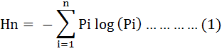
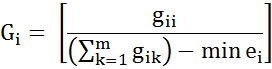
Where, Pi is the proportion of the built-up in the ith concentric circle. If the distribution is maximally concentrated, the Shannon’s Entropy (Hn), of zero is obtained. If distribution is evenly among the concentric circles, Hn will have maximum of log n.
Computation of spatial metrics: Spatial metrics are helpful to quantify spatial characteristics of the landscape. Select spatial metrics with details given in Table 2, were computed to analyse and understand the urban dynamics through FRAGSTATS (McGarigal and Marks in 1995) at three levels: patch, class and landscape levels.
 Range 0 to 1
 Range: ED > 0