Ramachandra. T.V ^1,2,3,*, Bharath H. AITHAL², Sowmyashree M.V^1
1Energy & Wetlands Research Group, Center for Ecological Sciences [CES]
²Centre for Sustainable Technologies (astra)
³Centre for infrastructure, Sustainable Transportation and Urban Planning [CiSTUP] Indian Institute of Science, Bangalore, Karnataka, 560 012, India
^*Corresponding Author: cestvr@ces.iisc.ernet.in

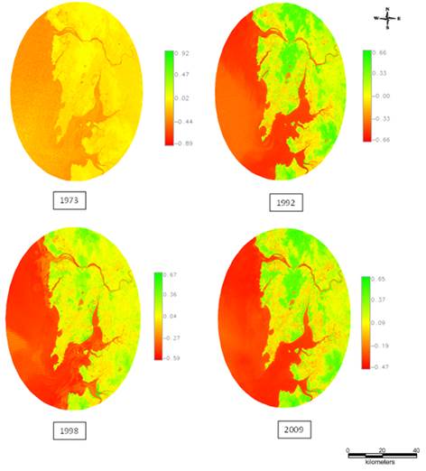
Results

5.1 Land Cover Analysis: Land cover analysis was performed using NDVI and results are provided in   Figure 4.NDVI ranges from -1 to 1. The negative value indicates the presence of non-vegetation such as built-up, water, sand etc. The positive values indicate the presence of vegetation. Table 5 tabulates the results of NDVI analysis.

Figure 4: NDVI from Landsat 1973, 1992, 1998 and 2009 for Mumbai region.

NDVI generated indicates that there has been a loss of green cover in the study region. Vegetation declined from 53.63 (1973) to 33.76 % (2009). There has been a loss in vegetation up to 62.79% during the past four decades. Vegetation class includes forests, agriculture, plantation, etc.  Land use analysis would help in getting details under each land use category.

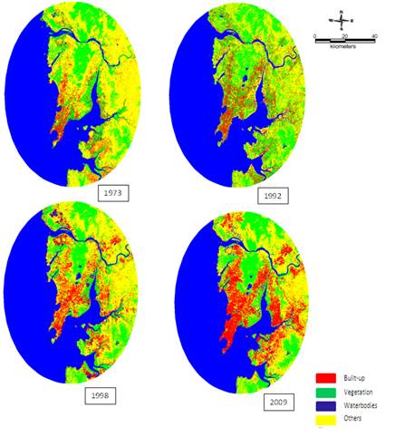
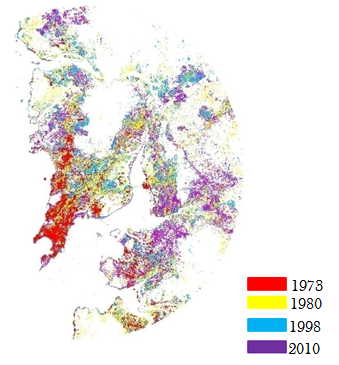
Table 5: NDVI output generated results gives idea about vegetation versus non vegetation.

5.2 Land use analysis: Temporal remote sensing data of the study area were classified using GMLC with training data. Data that was kept for validation were used to generate another set of classified images. Accuracy assessment of both the sets of classified images was done using error matrix, overall accuracy and Kappa statistics.  Figure 5 shows the classified images of the study region. Table 6 lists details of land use categories and Table 7 provides the overall accuracy and Kappa statistics of the classified data.

Land use statistics, as tabulated in table 6, indicates that there has been a phenomenal growth of urban area of 155% during the past four decades. Figure 6 depicts the process and diffusion of urban pockets in the study region during the past four decades. Further, the study area was divided into 4 zones and into concentric circles of 1km radius from the city centre. Figure 7 depicts the circle-wise land use statistics.

Figure 5: Spatial extent of land use categories in Mumbai

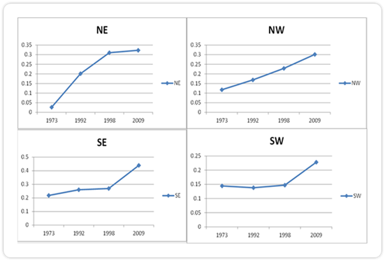
5.3 Shannon’s entropy (Hn): Table 8 lists the Shannon’s entropy calculated for the data of 1973 to 2009.  Figure 8 indicates the direction-wise Shannon’s entropy. This shows an increasing trend for NE and SW directions which indicates that urban patches are getting fragmented in time. In NW direction, Shannon’s entropy values show an increasing trend till 1998 that slightly decreases in 2009 indicating compactness. In SE direction, there has been an increasing trend from 1973 to 1992 with a sudden decline in 1998 (which shows compactness) and a slight increase in 2009 with increasing fragmentation.

Table 6: Land Use statistics of the classified images

Table 7: Overall Accuracy and kappa statistics of classified images

Table 8: Shannon’s entropy for Mumbai region.

Figure 6: Urbanisation pattern of Mumbai in past 4 decades

Figure 7:  Circle-wise land use statistics for Mumbai

Figure 8:  Shannon’s entropy for year 1973 to 2009.

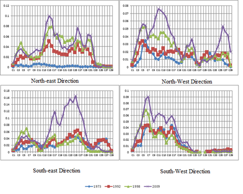
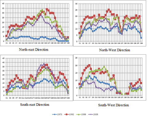
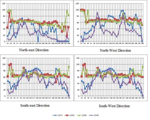
5.4 Spatial metrics analysis:
5.4.1 Percentage of landscape (PLAND):  PLAND (Figure 9a) equals the percentage of landscape comprised of the corresponding class patches. Built up percentage was computed to understand the ratio of built up and its increase in the landscape. Percentage of landscape gives a similar trend as the class area. In northeast direction, maximum PLAND is depicted in C13, C17, C25 and C27 in 2009. In northwest direction, the maximum value was found in C11, C12, C13, C14 and C15. Similarly, in SE (C13 to C27) and in SW (C5 to C21), the landscape comprised of high rate of urban patches as depicted in the graph below.

5.4.2 Number of patches (NP): Number of patches (NP) equals the number of built up patches in hectares in a landscape. It indicates the level of fragmentation in built up landscape (Figure 9b). In NE direction, C19 and C27 show a greater number of urban patches which imply that the patches are getting fragmented (more values found in 1992 and 1998 compared to 2009, whereas 1973 has a very low value which indicates the compact features of urban patches). In NW direction, the number of patches is varying for all circles (more variation is found in 1992 and 1998 compared to 2009, whereas, 1973 has a very low value which indicates the compact features of urban patches). In SE and SW directions, the number of patches is low which indicates the compactness of patches except for circles (C21 to C29) in southeast direction (i.e., maximum values found for the year 2009 indicates fragmentation).
Note: X axis indicates circles considered, Y axis value of the metrics

Figure 9a: PLAND direction and Circle wise

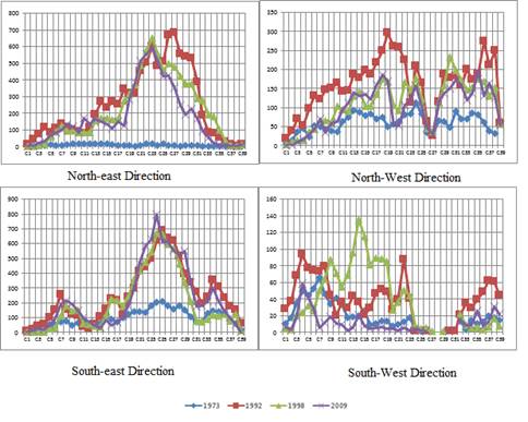
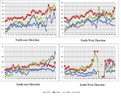
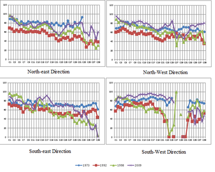
Figure 9b: metric NP direction and Circle wise

5.4.3 Patch Density (PD): Patch density (Figure 9c) is an indicator of urban fragmentation and as the number of patches increases, patch density increases which connotes to higher fragmentation. The metric shows results similar to the number of patches. In NE direction, C19 and C27 show more number of urban patches which connotes that patches are getting fragmented in time and hence higher values for the patch density were noticed in 1992 and 1998 (compared to 2009, whereas, 1973 has a very low value which indicates the compact features of urban patches). In NW direction, patch density is varying for all circles (more variation of values were found in 1992 and 1998 compared to 2009, whereas, 1973 has a very low value which indicates the compact features of urban patches). In SE and SW directions the patch density is low which connotes to the compactness of patches except for circles (C21 to C29) in SW direction.

5.4.4 Largest patch index (LPI): Largest Patch Index (LPI) was computed to represent the percentage of landscape that contain the largest patch (Figure 9d). The NE and SW directions show that the largest urban patches for the circles C13 to C20 indicating a less number of urban patches connoting to compactness of urban features (i.e., mostly in 2009). In NW and SW directions, the bigger urban patches are largely present towards the city center, connoting to more compact urban patches (i.e., circles from C1 to C17 showing maximum values for all years).

Figure 9c: PD direction and Circle wise

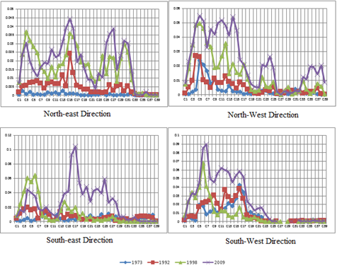
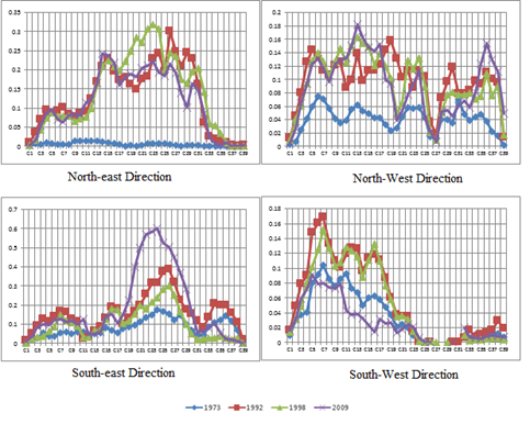
Figure 9d: LPI direction and Circle wise

5.4.5 Landscape shape index (LSI): Landscape shape index (Figure 9e) provides a simple measure of class aggregation or clumpiness and is measured via class edge surfaces.  Fig 9e depicts complex structure of urban patches that are found in mid circles (circles 10 to 19) compared to the circles present in urban center and fringes. In the NE direction, the metric value is less for the year 1973 for all circles indicating a simple structure and compact shapes, whereas, the years 1992, 1998 have maximum values compared to 2009 which implies that 2009 has compact patches compared to 1992 and 1998. Similarly, the NW direction shows a similar trend as the NE direction, i.e., 1973 shows compact features and 1992, 1998 have maximum values compared to 2009, indicating more fragmentation in the years 1992 and 1998 for all circles. The SE direction also shows a similar trend as the NE and NW direction. In SW direction, the urban patches show a simple structure for 2009 compared to 1992 and 1998 in all circles.

5.4.6 Normalized Landscape Shape Index (NLSI):  Normalized Landscape Shape Index (Figure 9f) is similar to landscape shape index but this represents the normalized value. This index provides a simple measure of class aggregation or clumpiness. Figure 9f below depicts the variations in the value and indicates that complexity of urban patches increases as it moves away from the core area. The analysis showed that the circles at the centre in 2009 were clumped compared to 1973, whereas circles (circle 28 onwards) show a characteristics of fragmented growth towards 2009.

Figure 9e: PD direction and Circle wise

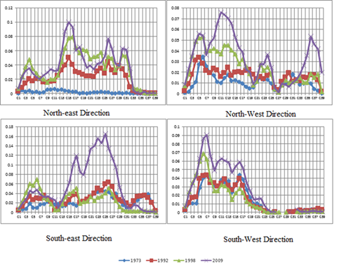
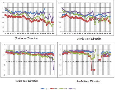
Figure 9f: NLSI direction and Circle wise

5.4.7 Edge Density (ED): Edge Density (Figure 9g) computes the total amount of edge present in a landscape. Edge Density (ED) represents the ratio of total edges of all the patches to total area. With increase in fragmentation, the number of patches increases and so does the number of edges. Hence edge density is the measure of fragmentation of the landscape. Figure 9g indicates that the edge density has maximum value for the circles C11 to C29 indicating greater fragmentation (i.e., greater values found in 1992 and 1998 compared to 2009, whereas, 1973 has a very low value which indicates the compact features of urban patches). In NW direction, maximum values for all circles were found in the year 1992 and 1998 compared to 2009 indicating greater fragmentation in 1992 and 1998 compared to 2009. In SE and SW directions, the number of patches is low which connotes to the compactness of patches, except for circles C21 to C29 in 2009 in SE direction which indicate fragmentation.

5.5.7 Clumpiness index (CLUMPY): Clumpiness index (Figure 9h) is the measure of patch aggregation. It measures the clumpiness of the overall urban patches. Clumpiness ranges from -1 to 1 where clumpiness is equal to -1 when the urban patch type is maximally disaggregated. Clumpiness is equal to 0 when the patch is distributed randomly and clumpiness approaches 1 when urban patch type is maximally aggregated. The graph shows that the value ranges from 0 to 1 which implies that the patches are getting aggregated in time for northeast and northwest directions. SE and SW directions also show a similar trend but C39 (SE) and C23, C25 (SW) show values of -1 indicating maximum disaggregation of urban patches.

5.4.8 Interspersion and Juxtaposition Index (IJI):  The Interspersion and Juxtaposition Index (IJI) (Figure 9i) measures the extent to which patch types are interspersed (not necessarily dispersed). Higher values result when the urban patch types are well interspersed (i.e., equally adjacent to each other), whereas lower values characterize landscapes in which the patch types are poorly interspersed (i.e., disproportionate distribution of patch type adjacencies) (McGarigal and marks, 1994). These metrics’ analysis showed same results as that of the clumpiness index, stating that the lower values are found in the inner circles in 2009 and higher values were near the boundary (circles 7 to 27).

5.4.9 Aggregation Index (AI):  Aggregation Index (Figure 9j) gives the similar indication as clumpiness i.e., it measures the aggregation of the urban patches. The aggregation index showed the similar trend as the clumpiness index. The aggregation index has maximum value at the city center and urban patches get disaggregated for the circles away from the city center as depicted in figure 9j.

Figure 9g: ED direction and Circle wise

Figure 9h: ED direction and Circle wise

Figure 9i: IJI direction and Circle wise

Figure 9j: AI direction and circle wise